Gapology

In this work, we investigated the possibility that globular clusters can create gaps in the Palomar 5 stellar stream. This project began during the development phase of our code, when we first introduced perturbers. Initially, we intended these perturbers to represent dark matter subhalos or giant molecular clouds. However, before generating a new dataset, we tested the code using the catalog of globular clusters. To our surprise, we found that several clusters produced clear gaps in the Palomar 5 stream, which motivated us to carry out a detailed analysis. Here, we report the frequency of interactions that generate significant gaps, and identify the clusters responsible for these perturbations. Finally, in the supplementary material, we discuss the persistence of these gaps in light of the velocity distribution within the stream.

Introduction

Stellar streams are several-kiloparsecs-long structures formed by the tidal disruption of globular clusters or dwarf galaxies orbiting a host galaxy. These tidal forces arise due to differential gravitational pulls across extended objects, causing stars farther from the galactic center to lag behind, while those closer to the center speed up. This stretching creates two tidal tails that trace the cluster’s orbit unless in the closest vicinity to the object (Montuori et al. 2007).

Numerical predictions of this phenomenon have existed since the 1970s (see, e.g., Keenan and Innanen 1975). These predictions occurred well before the first detections of Galactic globular cluster tidal tails (Carl J. Grillmair et al. 1995). Interestingly, Carl J. Grillmair et al. (1995)’s detections were made nearly contemporaneously with the discovery of the Sagittarius stellar stream by R. A. Ibata, Gilmore, and Irwin (1994), which is the closest example of a stream emerging from a dwarf satellite currently interacting with the Milky Way.

Subsequent studies¹ extended Grillmair’s findings to other globular cluster streams but were often limited to the detections of stars still close to the cluster tidal radius, until the discovery made by Michael Odenkirchen et al. (2001, 2003; M. Odenkirchen et al. 2002) of long and thin tails outside the Palomar 5 globular cluster. With a mass of \(1.34\pm 0.24 \times 10^4 M_{\odot}\) (Baumgardt et al. 2019), Palomar 5 is one of the least massive globular clusters in the Galaxy. Michael Odenkirchen et al. (2003) showed that its tails contain more mass than the cluster. The works of C. J. Grillmair and Dionatos (2006a) and Kuzma et al. (2015) showed that the tails have an extent of more than \(20^\circ\) degrees in the sky. The discovery of its prominent tails stimulated a vigorous and successful search in the following years. New streams were discovered, mostly taking advantage of Sloan Digital Sky Survey data, but Pan-STARRS and ATLAS were also used (C. J. Grillmair and Dionatos 2006b; Belokurov et al. 2006; C. J. Grillmair 2009, 2014; Bonaca, Geha, and Kallivayalil 2012; Carl J. Grillmair et al. 2013, 2015; E. J. Bernard et al. 2014; Edouard J. Bernard et al. 2016; Carl J. Grillmair 2017; Koposov et al. 2014).

Bonaca and Price-Whelan (2025) provides a review of stellar stream astronomy, which has entered a new era since the publication of the data from the Gaia astrometric mission (Gaia Collaboration et al. 2016). Gaia’s characterization of billions of stars in the Milky Way enables the search for these structures by coupling photometry, astrometry, and spectroscopy for the brightest stars. The possibility given by Gaia to track stars with coherent movements over the entirety of the sky has led to the discovery of dozens of new streams. In addition, Malhan and Ibata (2018) developed the streamfinder algorithm and applied it across a series of works (Malhan, Ibata, and Martin 2018; Rodrigo A. Ibata et al. 2018; Rodrigo A. Ibata, Malhan, and Martin 2019) to discover a multitude of streams.

The possibility of combining Gaia data with spectroscopic surveys has extended the study of stellar streams beyond the quantification of their orbital properties to a full chemical characterization (T. S. Li et al. 2019; Ji et al. 2020; Ting S. Li et al. 2021, 2022; Usman et al. 2024). Currently, about a hundred stellar streams are known in our Galaxy. Mateu (2023) compiled their tracks on the sky into a catalog. Interestingly, only about 20 streams are associated with known Galactic globular clusters.

One of the interests in studying stellar streams is that they can constrain the gravitational field of their host galaxies, particularly the Milky Way. Compared to the measurement of the HI rotation curve, stellar streams offer the opportunity to investigate the potential of the host galaxy over a wide range of distances, reaching the outermost regions of the halo. For example, Varghese, Ibata, and Lewis (2011) demonstrated how stellar streams can be used to infer the mass and scale parameters of dark matter halos, utilizing various amounts of observational data, ranging from basic right ascension and declination to full six-dimensional phase space information. Bonaca and Hogg (2018) reviewed this concept from an information-theoretic point of view, identifying which orbits and configurations of stellar streams yield the most information about the Galactic potential. However, using single streams to constrain the potential led to ambiguous and non-converging results. For example, Law and Majewski (2010) made use of the Sagittarius stream to infer that the dark matter halo of our Galaxy has a triaxial shape (see also Helmi 2004; Johnston, Law, and Majewski 2005; Law, Johnston, and Majewski 2005), but Bovy et al. (2016) concluded that the dark matter halo of our Galaxy is nearly spherical at the distances of the Palomar 5 and GD-1 streams. The two contrasting results could indicate that the halo is triaxial at one distance but spherical at another, highlighting the need for streams at different distances to map the halo shape. Recently, R. Ibata et al. (2024) constructed a Milky Way model by applying a Markov chain Monte-Carlo (MCMC) fitting procedure. This method identified the set of potential parameters in an axisymmetric model of the Milky Way that best reproduces all observed stellar streams.

Beyond the global visible and dark mass distribution streams, streams can also be used to infer the granularity of the dark matter, that is, the mass and density of the subhalos populating our Galaxy. According to simulations by Springel et al. (2008), the \(\Lambda\) cold dark matter (\(\Lambda\)CDM) model predicts that galaxies grow hierarchically, with dark matter clumps forming at a wide range of masses and sizes. These clumps, or subhalos, are predicted to follow a mass distribution with a power-law slope slightly shallower than -2.0. Vegetti et al. (2012) detected the smallest observed dark matter halo through gravitational lensing in an Einstein ring with a mass of \(10^8\) solar masses. However, some models predict that dark matter clumps could exist down to at least the mass of Earth-like planets (Green, Hofmann, and Schwarz 2005; Amorisco 2021, see).

R. A. Ibata et al. (2002) first suggested that dark matter subhalos could influence stellar streams by diffusing their orbital elements. Later, Carlberg (2012) expanded this idea, proposing that subhalos could create gaps in stellar streams during flyby encounters, where a subhalo approaches closely enough to a segment of a stream and significantly changes the orbits of the closest stars. Carlberg and Grillmair (2013) applied this idea and looked for the presence of gaps in the well-known Palomar 5 and GD-1 streams, concluding that the density variations found in their streams were consistent with expectations from \(\Lambda\)CDM models. Bonaca et al. (2019) provided further observational evidence for this idea, identifying a gap and a spur in the GD-1 stream that they could not explain by known objects, such as globular clusters, and which they suggested was due to the close passage of a dark matter subhalo. Interestingly enough, as stated in Bonaca et al. (2019), the recovered properties of this subhalo (mass and size) were denser than those with the \(\Lambda\)CDM mass-size relationship presented in (Moliné et al. 2017). The works mentioned are only a few examples of the extensive literature that has explored the impact of dark matter subhalos in simulated streams (Helmi and Koppelman 2016; Hermans et al. 2021; Banik et al. 2021; Hilmi et al. 2024; Nibauer et al. 2025) or searched for their traces in observed streams (Thomas et al. 2016; Erkal, Koposov, and Belokurov 2017; Bonaca, Pearson, et al. 2020; Bonaca, Conroy, et al. 2020).

In contrast, a limited number of works have explored whether other structures, such as those from baryonic matter, can cause variations in the density of streams and gaps that can be confused with those produced by dark matter subhalos. Among these works, it is worth mentioning the results of Pearson, Price-Whelan, and Johnston (2017), which suggest that the presence of the bar at the center of the Galaxy can perturb the characteristics of a stream, such as Palomar 5, and generate gaps along its tail. That the Galactic bar could have an influence on stream morphology was also discussed by Hattori, Erkal, and Sanders (2016) and Price-Whelan et al. (2016), in the case of the Ophiuchus stream (E. J. Bernard et al. 2014). Besides the Galactic bar, giant molecular clouds can also produce gaps in stellar streams, as shown by Amorisco et al. (2016). All of these works thus indicate that baryonic structures can play an important role in tail morphology. In this context, an extensive numerical study specifically focused on modeling the tails of Palomar 5 under the influence of the Galactic bar, spiral arms, giant molecular clouds, and globular clusters, has been realized by Banik and Bovy (2019), who concluded that both the influence of the bar and that of the giant molecular clouds can leave imprints on Palomar 5 tidal tails similar to those left by dark matter subhalos. In contrast, they found the effect of globular clusters to be negligible.

Few studies have specifically investigated the effect of globular clusters on stellar streams. Erkal, Koposov, and Belokurov (2017) concluded that globular clusters could not be responsible for the observed density variations in the tails of Palomar 5. Their analysis focused on the characteristics of the observed gaps and involved constraining progenitor properties using reconstructive modeling. By trial and error, they identified a specific configuration of masses, sizes, impact parameters, times of impact, and relative velocities for two perturbers that successfully reproduced the observed density distribution. However, as we do in this work, their method does not perform full forward modeling of the entire globular cluster system on Palomar 5’s stream. While they suggest that the impact rate of globular clusters is likely less significant—given their lower abundance compared to the expected dark matter subhalos population—they do not explore this aspect in detail. However, they state that it is an avenue for future investigation.

More recently, Doke and Hattori (2022) have examined the possibility that gaps in the GD-1 stellar stream could be due to the close passage of globular clusters, concluding that this scenario is improbable. These first works suggest that the impact of globular clusters on stellar streams is negligible. This result does not necessarily need to be the general case, especially for streams of clusters such as Palomar 5, which live in the inner 20 kpc of the Galaxy, where many other globular clusters also orbit. For example, Khoperskov et al. (2018), Alessandra Mastrobuono-Battisti et al. (2019), and Ishchenko, Sobolenko, Berczik, Omarov, et al. (2023) showed that globular clusters can even collide with other clusters, which implies that cluster stream collisions should happen much more frequently since streams are far more extended than clusters.

In this study, we aim to fill this gap in the literature on numerically modeling cluster-stream interactions. We seek to quantify the impact of passing globular clusters in the vicinity of streams to understand whether these systems can also be effective and how frequently they alter the distribution of stars in the tails, producing underdense regions or gaps. To this end, in the following pages, we present the results of simulations of the streams of Palomar 5 subject to the gravitational interaction with the set of 165 Galactic globular clusters for which positions and velocities are known to date and for which orbits can therefore be reconstructed (Baumgardt and Vasiliev 2021). We chose to simulate streams formed from a cluster with the current characteristics of Palomar 5 because it is a halo cluster with extended tails, and because it is a cluster for which the effect of baryonic structures on its stream has already been studied. As we show, and in tension with previous claims, the close passage of other clusters with such a stream is not rare. Indeed, in the 50 simulations we ran, we found the formation of numerous gaps, averaging 1.5 gaps per simulation, generated by 18 different clusters across the entire system of Galactic globular clusters.

Methods

The most accurate model of the Palomar 5 stream would involve full modeling of the internal dynamics of the cluster, which would mean computing \(N\)-body interactions with a \(\mathcal{O}(N^2)\) computation time, stellar evolution, supernovae, an initial mass distribution, treatment of binary star systems, etc. (for such an example, see Gieles et al. 2021; Wang et al. 2016). Instead, we opt for solving the restricted-three-body problem, also known as the particle-test method, as we did for Ferrone et al. (2023), which we describe here for completeness. As demonstrated by A. Mastrobuono-Battisti et al. (2012), although the restricted three-body problem neglects the internal evolution of the cluster, it still reproduces very similar stream properties since the model captures key extracluster physics, such as disk shocking and epicyclic stripping.
Below, we first present the approach used to include the Galactic globular cluster system in our modeling (Sect. 2.1), highlighting the similarities and differences with respect to what we did in Ferrone et al. (2023); we then summarize the method used to model the mass loss from the cluster (Sect. 2.2) and finally discuss the quality of the numerical integration (Sect. 2.3).

Numerical methodology

We begin by extracting positions in the sky, proper motions, line-of-sight velocities, and distances, as well as masses and half-mass radii, of 165 globular clusters from the Galactic globular cluster catalog by (Baumgardt and Vasiliev 2021).² We then convert the initial conditions from sky coordinates into a Galactocentric reference frame, by adopting a velocity for the local standard of rest of \(v_{\text{LSR}} = 240\) km s\(^{-1}\) and a peculiar velocity of the Sun equal to \((U_\odot, V_\odot, W_\odot)=(11.1, 12.24, 7.25)\) km s\(^{-1}\), as reported by Schönrich (2012). We set the Sun’s position to \((x_\odot,y_\odot,z_\odot) = (-8.34,0,0.027)\) kpc. We took the vertical position above the disk from Chen et al. (2001) and the distance of the Sun to the Galactic center from Reid et al. (2014). These transformations were performed using astropy (Astropy Collaboration et al. 2013).

For the Galactic potential, we employed the second model from Pouliasis, Di Matteo, and Haywood (2017), a superposition of a thin disk, thick disk, and dark matter halo, with masses and scale lengths provided in Table 1 of Ferrone et al. (2023). This model is time-independent throughout our simulations. This model satisfies a series of observational constraints such as local solar, stellar density, the Galactic rotation curve, similarly to other Galactic models such as MWpotential2014 from Bovy (2015) and McMillian2017 from McMillan (2017). However, we use only one Galactic potential to balance data volume and computation time, which should suffice. Vasiliev and Baumgardt (2021) found that only a few outer globular clusters are strongly affected by different potential models. Generally, kinematic uncertainties are the dominant factor in differences between orbital solutions per cluster. Similarly, Grondin et al. (2024) generated a globular cluster mass-loss catalog using seven different potential models and found that their debris distributions were rather model-independent, similar to those of Ferrone et al. (2023). While the clusters’ exact positions in time may depend on the model, we assert that interaction rates and stream formation are largely independent of the choice of the Galactic potential model.

Lastly, we select an integration time of 5 Gyr as a compromise between maximizing interaction statistics and modeling the Galaxy as a time-independent, constant mass distribution. Ishchenko, Sobolenko, Berczik, Khoperskov, et al. (2023) analyzed the orbits of the Galactic cluster population using the same initial conditions as in this work within five live Milky Way-like potentials from IllustrisTNG (Pillepich et al. 2018). They found that in all sampled potentials, orbital changes remain minimal over 5 Gyr, becoming significant only at earlier look-back times when the host galaxy had significantly less mass or was undergoing a merger event.

Full simulations

There is a primary methodological departure from Ferrone et al. (2023). In that work, globular clusters evolved under the gravitational effect of the Galaxy alone. In contrast, now we also consider the effect of all other Galactic globular clusters by taking into account the direct \(N\)-body interactions between them. First, all clusters are represented by Plummer spheres, each with its own mass and half-mass radius as reported in the Baumgardt catalog (Baumgardt and Vasiliev 2021). For the remainder of this paper, the full simulations consider the gravitational forces from the globular cluster interactions.
For these simulations, we proceeded in two steps:

The procedure described so far has been repeated 50 times, generating a new set of initial conditions each time, given the uncertainties on proper motions, line-of-sight velocities, distances to the Sun, and masses of all clusters, as reported in the Baumgardt catalog. We handle these uncertainties through a Monte-Carlo approach by sampling them with a Gaussian distribution and considering the covariance term between the proper motions. We use the most probable values for the initial conditions in the first simulation. We sample the uncertainties for all globular clusters. Additionally, for each resampling of Palomar 5’s mass, we also resample the distribution of the 100,000 star particles.

During the integration, we save intermediate snapshots to facilitate the analysis of stellar streams and the effects of cluster impacts. Specifically, for each realization of the Palomar 5 stream, we saved \(5000\) in snapshots, equivalent to a temporal resolution of 1 million years. We provide the parameters that specify our data volume in Table 1. Using single precision floating point numbers, the size of our simulations is approximately: \[\label{eq:data_volume_estimate} N_p \times N_{\mathrm{ts}}\times N_{\mathrm{phase}}\times N_{\mathrm{sampling}} \times 4~\mathrm{bytes}\approx 600~\mathrm{Gb}.\]

Parameters determining the data volume. \(N_p\) is the number of particles, \(N_{\mathrm{ts}}\) is the number of time-steps saved, \(N_{\mathrm{phase}}\) is the number of phase space coordinates, and \(N_{\mathrm{sampling}}\) is the number of Monte-Carlo samplings of the initial conditions.
\(N_p\)	\(N_{\mathrm{ts}}\)	\(N_{\mathrm{phase}}\)	\(N_{\mathrm{sampling}}\)
\(100000\)	\(5000\)	\(6\)	\(50\)

Reference simulations

To quantify the impact of globular cluster passages on the density of the Palomar 5 stream, we performed a second set of simulations, which we refer to as the reference simulations in this paper. These reference simulations use the same 50 sets of initial conditions as the full simulations, the same Galactic potential, but exclude mutual interactions between globular clusters. The approach adopted for this second set of simulations is thus equivalent to that adopted already in Ferrone et al. (2023). In Eq. [eq:GCNBody], only the gradient of the Galactic potential is considered. In Eq. [eq:equation_of_motion_particle], of the second term on the right side of the equation, only the influence of Palomar 5’s Plummer sphere on Palomar 5’s particles is considered. In other words, the sum iterates over only one globular cluster, the host. We omit all interactions with the other clusters.

Mass loss

Each of the 100,000 particles that initially populate the cluster undergoes experiences the forces from Pal 5 and the Galactic potential. The mass and radius of Pal 5 are held constant over time. At each time step, a certain number of particles will therefore acquire sufficient energy to no longer be gravitationally bound to the cluster itself and thus go on to populate the streams, whose mass and spatial extent grow over time. It is important to note that in the approach used:

The assumption in point 2 is a direct consequence of the approach described in point 1. Starting from a cluster with a mass and size similar to the current ones can lead to streams with lower velocity dispersions than those we would obtain if we had used a self-consistent approach. In a future article, we will report on the study of gap survival times depending on the masses and sizes of progenitor clusters (Ferrone et al, in prep). We note, however, that simplifications of this kind are not uncommon in literature. Pearson, Price-Whelan, and Johnston (2017) discussed the formation of gaps in the Pal 5 tails and assumed a time-independent mass of \(50,000 ~\mathrm{M}_\odot\) for Pal 5, over the last 4 Gyr; Erkal, Koposov, and Belokurov (2017) adopted a N-body approach to simulate Pal 5 stream, but used Pal 5 current conditions as their progenitor’s initial conditions; Banik and Bovy (2019) simulated the Pal 5 stream as emerging from a stellar system with a velocity dispersion of 0.5 km/s (similar to that of particles escaping from our cluster, as we have verified).

The characteristics of the streams modeled in this paper may be considered more representative of those of clusters that are now completely dispersed, i.e., it is conceivable that completely dispersed globular clusters that left behind a population of ‘orphan’ streams passed through characteristics similar to those of Pal 5 today (small masses and extended radii). In this sense, the initial conditions chosen (in terms of internal parameters) may be more representative of those of streams for which the progenitor is now dissolved (see, for example, the population of streams without progenitors described by R. Ibata et al. 2024) than those currently typical of Galactic globular clusters than those currently typical of Galactic globular clusters. ⁴

Numerical stability

We used a leapfrog integrator because of its ability to preserve phase-space volume and conserve the Hamiltonian with each integration step. For instance, this method is preferable to a Runge-Kutta scheme, which can introduce non-physical and significant numerical errors in systems that require long-term stability and energy conservation. One drawback of the leapfrog integrator is that it requires a uniform time step throughout the entire computation, resulting in unnecessary computations for a particle after it has escaped from the host cluster. However, energy conservation and phase-space volume preservation are paramount when modeling stellar streams. The time step was therefore set to be small enough to conserve energy for the most interior particles within the cluster—ensuring that a higher mass loss did not arise from numerical error. We found that a time-step of 10,000 years was adequate to maintain energy conservation, with a median variation of \(10^{-12} \frac{\Delta E}{E_0}\), where \(E_0\) is a particle’s initial energy, and \(\Delta E\) is the difference between its final and initial energy.

We also checked the reverse integrability of the globular cluster system for the reference simulations. By reverse integrability, we mean the integrator’s capability to track the cluster backward in time and then re-integrate it forward along the same trajectory. Integrating point masses in a static axis-symmetric potential conserves \(L_z\) and \(E\), which create regular periodic and non-chaotic orbits. Therefore, any drift would arise from purely numerical error. We selected a timestamp for which the drift in the final position after forward integration, compared to the initial position from the backward integration, was consistently at least two orders of magnitude smaller than the Plummer scale radius used for Palomar 5. This high precision ensures that no fictitious numerical forces influence the system, preventing any artificial mass loss or retention of star particles.

Results

Overview

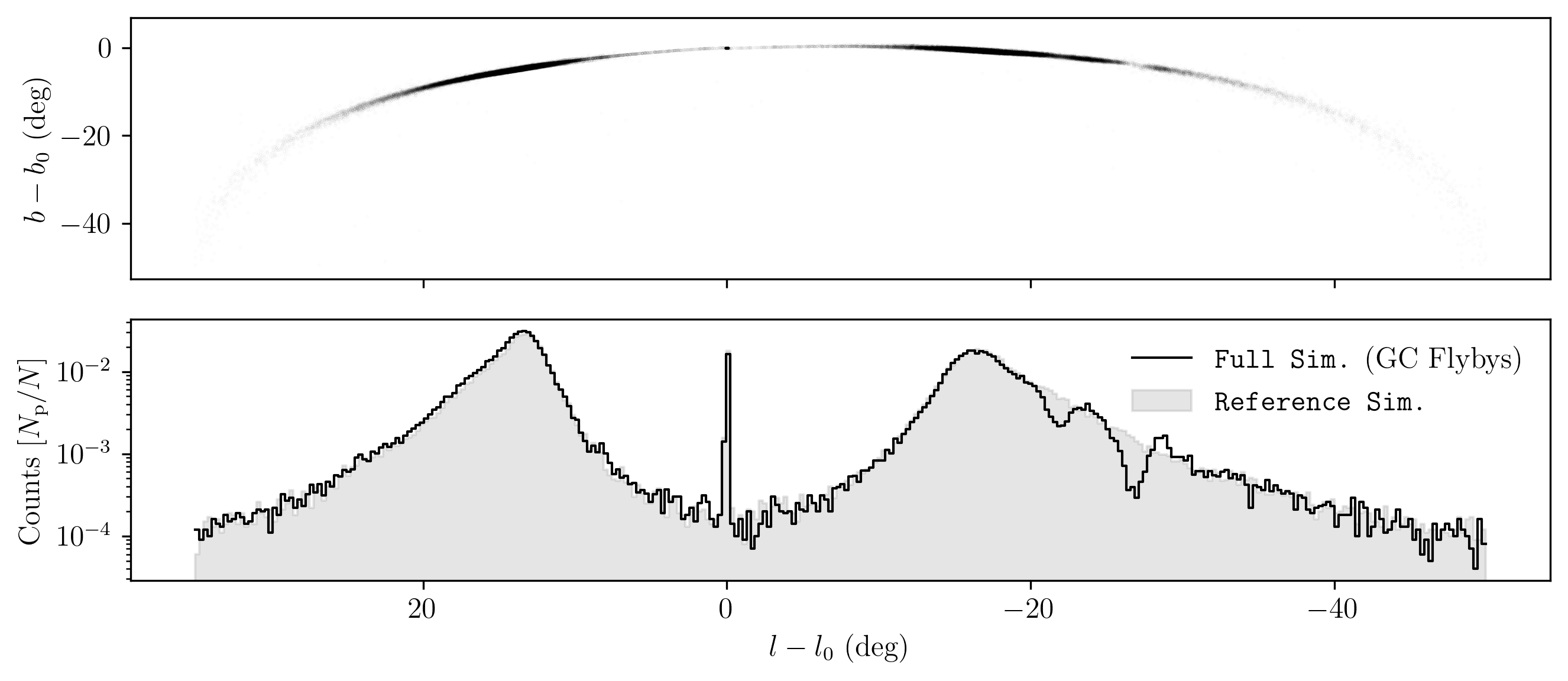
The presence of the other globular clusters affects the properties of the Palomar 5 stream. Fig. [fig:stream_on_sky] presents an obvious example of this effect, which we selected for its prominent gaps. Two of these gaps are visible in Galactic coordinates and become even more apparent when marginalizing over latitude to reconstruct the 1D density profile of the stream as a function of longitude.

Regarding the shape of the density distribution, the central peak corresponds to the still-intact globular cluster whose stars have not yet escaped. The stream’s density peaks are of the same order as the cluster itself, which is inconsistent with reality; the cluster’s peak density should be higher than that of the stream. Of course, this discrepancy is a result of our modeling choices. Since we use the present-day mass and radius for Palomar 5 for the whole simulation duration, the system is less dense than it should have been. In turn, our simulations have a strong initial mass loss, which adds to the amplitudes of the profile density peaks of Fig. [fig:stream_on_sky]. This inaccuracy is acceptable for the scope of this work. First, Palomar 5’s tails indeed have more mass than the cluster itself. Rodrigo A. Ibata et al. (2017) reports that there could be three times as much mass in Palomar 5’s tails as the cluster itself. Secondly, the exact form of the density distribution is less important than having a population of particles present that can probe a cluster flyby event.

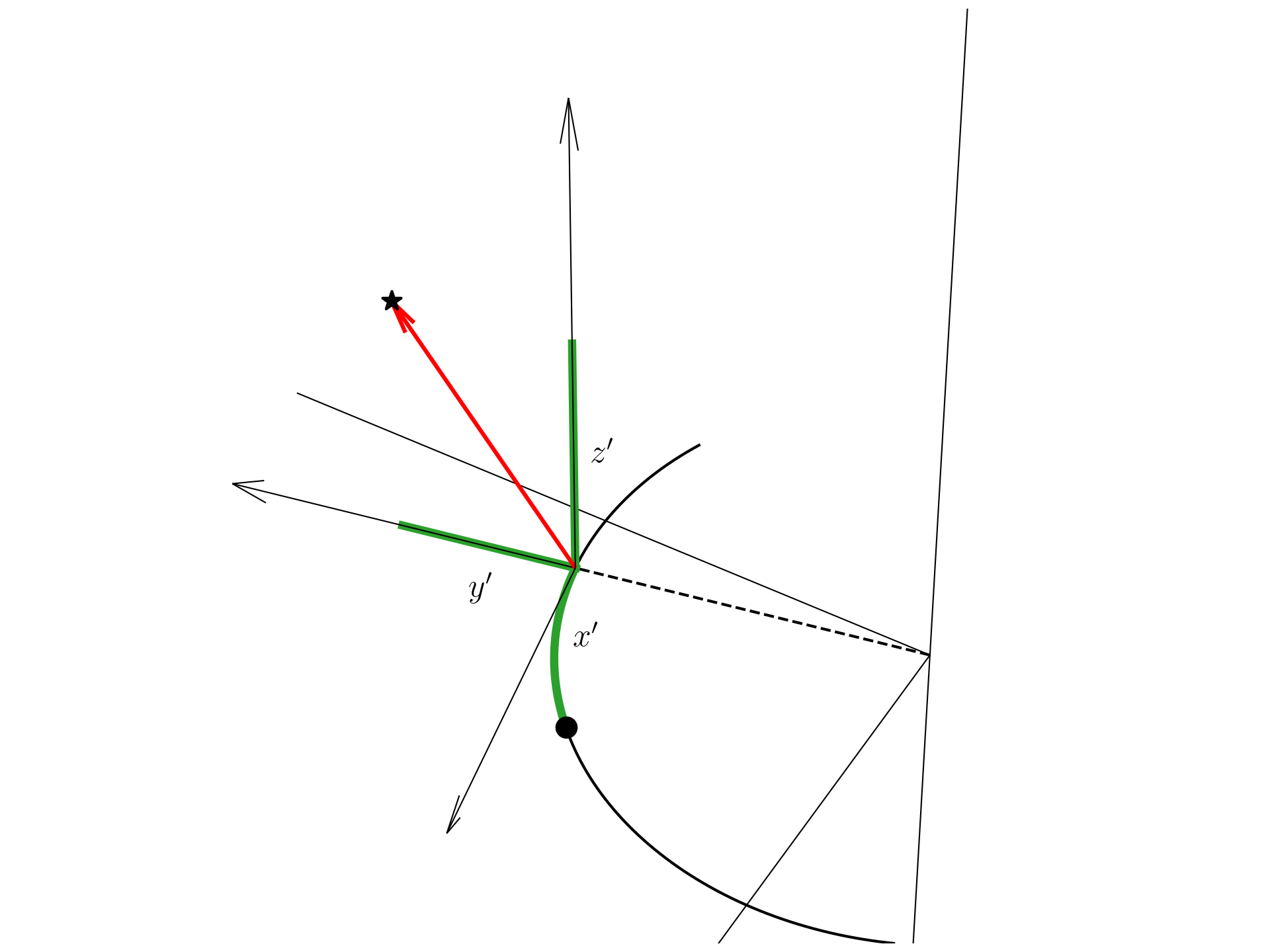
To compare the reference and full simulations more quantitatively, we work in the tail coordinate system, in which the stream’s central axis aligns with the cluster’s orbit. We based this coordinate system on the work of Dehnen et al. (2004) and present it in Fig. 4. Briefly, in this system, the \(x_{\mathrm{tail}}\) coordinate represents the position of a particle along the orbit relative to the globular cluster. Positive values of \(x_{\mathrm{tail}}\) are ahead of the cluster, while negative \(x_{\mathrm{tail}}\) is behind the cluster. 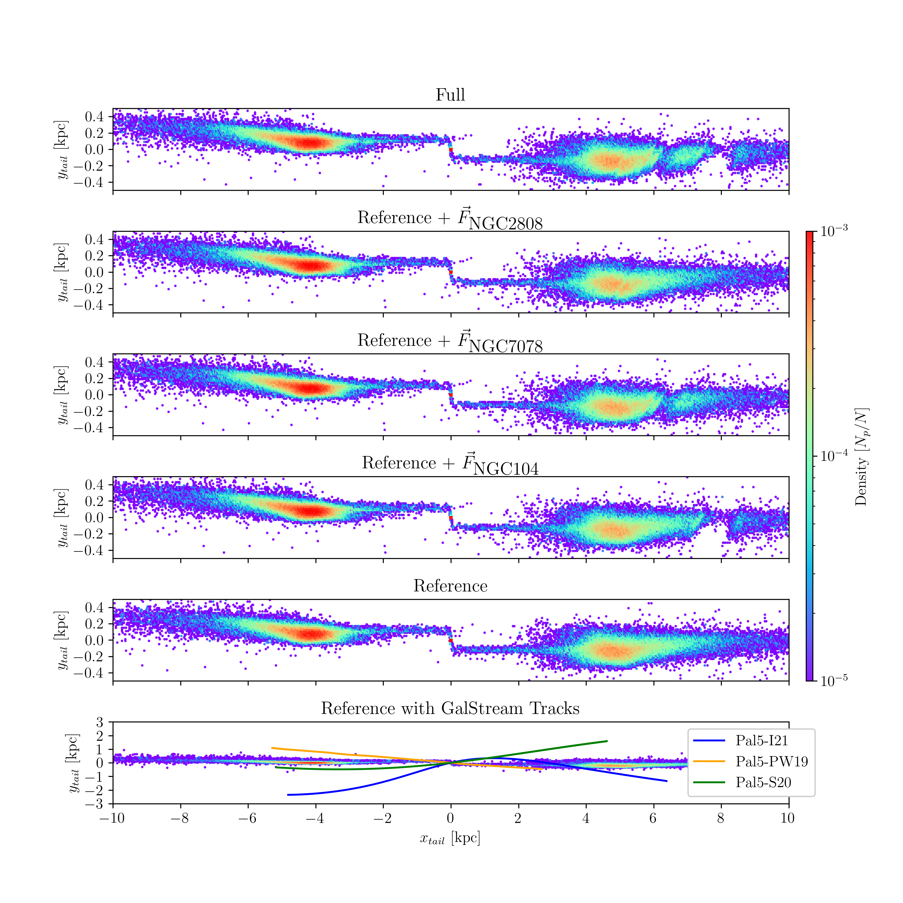The \(y_{\mathrm{tail}}\) coordinate measures the particle’s distance within the orbital plane, where positive values indicate that the particle is farther from the Galactic center and negative values indicate that it is closer. Fig. [fig:decomposition] shows a comparison between one of the 50 realizations of the Palomar 5 stream, taking into account the gravitational interactions with all other globular clusters in the Galaxy (top panel) and omitting them (bottom panel). This comparison clearly shows the presence of two wide (\(\sim\)100 pc and \(\sim\)1 kpc) gaps in the leading tail and of a more subtle underdensity at \(x_{\mathrm{tail}}\sim 5\) kpc (we refer the reader to Supplemental Material 6.1 for a detailed description of the underdensities and gaps detection method).

To determine which globular clusters were responsible for creating these gaps and when close passages occurred, we estimated the gravitational acceleration along the orbit of Palomar 5. We represented it in the (\(t\), \(\tau\)) space. \(t\) is the simulation time, and \(\tau\) indicates how long it will take for Palomar 5 to reach a given point in its orbit or how long ago it passed. The use of \(\tau\) is advantageous because the growth of the stream is approximately linear in \(\tau\).

On the other hand, streams in physical space are modulated by their orbital eccentricity with periodic expansion and contraction depending on the orbital phase (see the top panel of Fig. 5. Sanders, Bovy, and Erkal 2016, for an example). Adopting this time-space and reporting the gravitational acceleration along the Palomar 5 orbit in this space, identifying the globular clusters that produced the perturbation and the time at which it occurred becomes straightforward. We refer the reader to Supplemental Material 6.2 for a detailed description of the procedure. In this way, we can identify that the clusters responsible for creating gaps in the simulation of the Palomar 5 stream, as reported in Fig. [fig:decomposition], are NGC 2808, NGC 7078, and NGC 104. Their close passages occurred 200 Myr, -1.9, and -2.1 Gyr ago, respectively.

To further investigate whether the three clusters above are responsible for producing the gaps observed in this simulation, we conducted additional experiments by including only the perturbation of each cluster at a time, while neglecting the gravitational perturbations of all the other clusters in the Galaxy.

To verify that the three suspected clusters are responsible for producing the gaps, we conducted experiments by including one perturbed at a time and excluding all others. We present these results in the middle panels of Fig. [fig:decomposition] and clearly show that NGC 2808, NGC 7078, and NGC 104 are the clusters responsible for creating the underdense regions observed in the leading tails of Palomar 5. It is worth noting that the times at which the passages of these clusters occurred, according to our analysis, are in agreement with the observed width of the corresponding gaps: the encounter with NGC 2808 being very recent (only 200 Myr ago), its induced gap is still very thin, because it takes time for a perturbation to grow into an extended gap, as it is the case for those induced by the passages of NGC 7078 and NGC 104, which occurred in earlier times. It is also interesting to emphasize that gaps as thin as those generated by the passage of NGC 2808, 200 Myr ago, can be detected by working in the tail coordinate system and by making a comparative analysis (full versus reference simulations): they are so thin that they cannot be directly identified in Galactic coordinates (see Fig. [fig:stream_on_sky]).
The analysis presented in Fig. [fig:decomposition] has been repeated for the whole set of simulations, and online appendix reports all of them for completeness. For all the streams, morphologically speaking, the only changes appear to be the existence of gaps or their absence. We do not observe a thickening of the streams due to an increased velocity dispersion.

From this analysis, we can derive a statistical view of (1) the number of gaps generated on the Palomar 5 stream by the system of Galactic globular clusters, (2) the clusters that generated these gaps, and the time history of these perturbations. From this, we can then quantify (3) the properties of the perturbers (their masses, sizes, and orbital parameters) as well as (4) the impact geometry of the encounters, which allows us to understand which encounters are more favorable for generating gaps in the Palomar 5 stream. In the following, we will present the results of this analysis, addressing points (1) and (2).

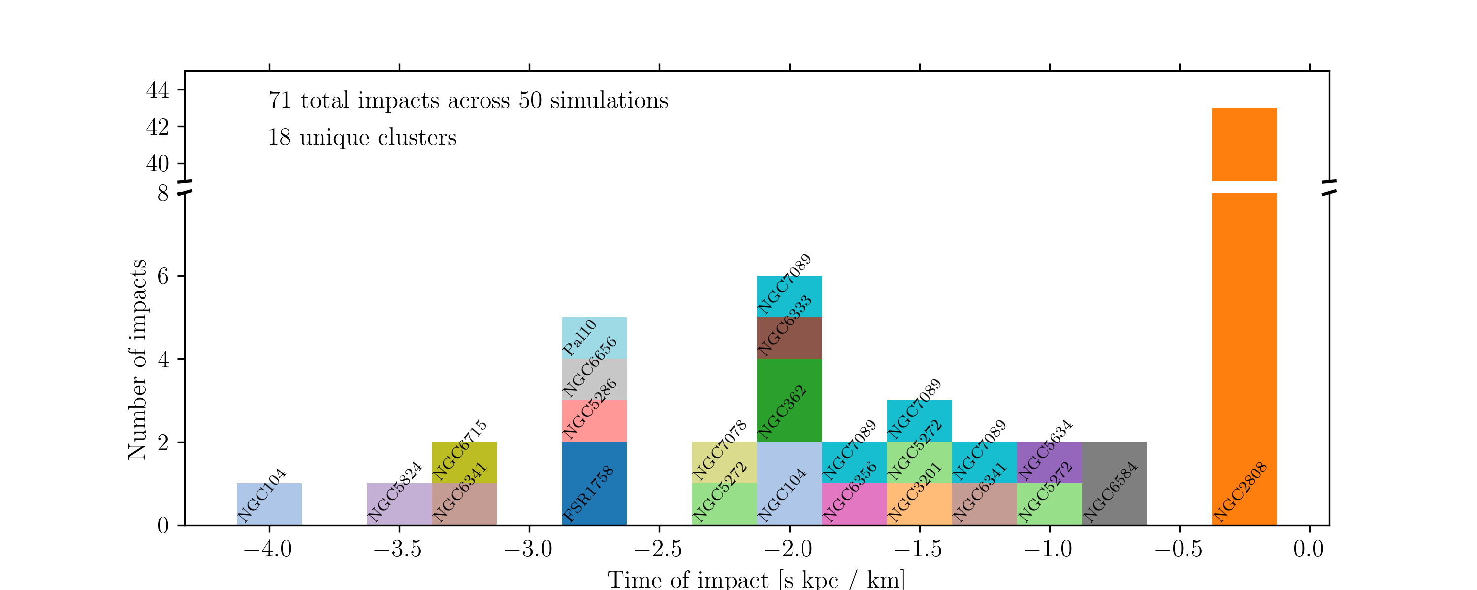
The history and statistics of gap creations in the Palomar 5 stream

By applying the methodology described above to the whole set of simulations, we can reconstruct the history of close passages of Galactic globular clusters to Palomar 5’s stream in the last 5 Gyr, which – we remind the reader – is the time interval investigated in our simulations. Fig. [fig:histogram_impact_time] and Table 2 present results of this analysis. NGC 2808 impacted Palomar 5’s stream about 200 Myr ago in 44 out of 50 simulations, creating a small gap at a similar position to the one reported in Fig. [fig:decomposition] in each case. Since this interaction occurred less than one orbital period ago, despite the uncertainties, the orbital solutions remain similar and thus produce consistent results across all simulations. However, as we continue to turn back time further, the uncertainties in the initial conditions allow the various orbital solutions to diverge from one another. Thus, in one configuration, a cluster can impact the stream at a given time, and yet at the same moment, in a different set of initial conditions, it could be on the other side of the Galaxy. We will discuss the necessary conditions for creating a gap in Supplemental Material 6.4.

Number of gaps created by each perturber across all 50 simulations. These data are color-coded and illustrated in Fig. [fig:histogram_impact_time].
NGC2808	44	NGC7089	5	NGC5272	4
NGC6584	3	NGC6341	2	NGC6656	2
NGC104	2	NGC3201	1	NGC5634	1
NGC5286	1	NGC362	1	NGC5824	1
NGC6356	1	NGC6333	1	NGC6715	1
FSR1758	1	NGC7078	1	Pal10	1

In total, we report the finding of 73 gaps across our 50 simulations, which averages to 1.5 gaps per simulation. Eighteen different perturbers provoke the gaps. Table 3 presents the distribution of the number of gaps appearing per simulation. If we consider NGC 2808 an outlier and exclude it from the experiment, we observe an average of 0.6 gaps per simulation.

Occurrence of gaps in Palomar 5 streams, in our simulations. More specifically, the table reports the number of simulations (second row) for a given number of gaps (first row).
Number of Gaps	0	1	2	3	4
Number of Sims.	4	25	16	4	1

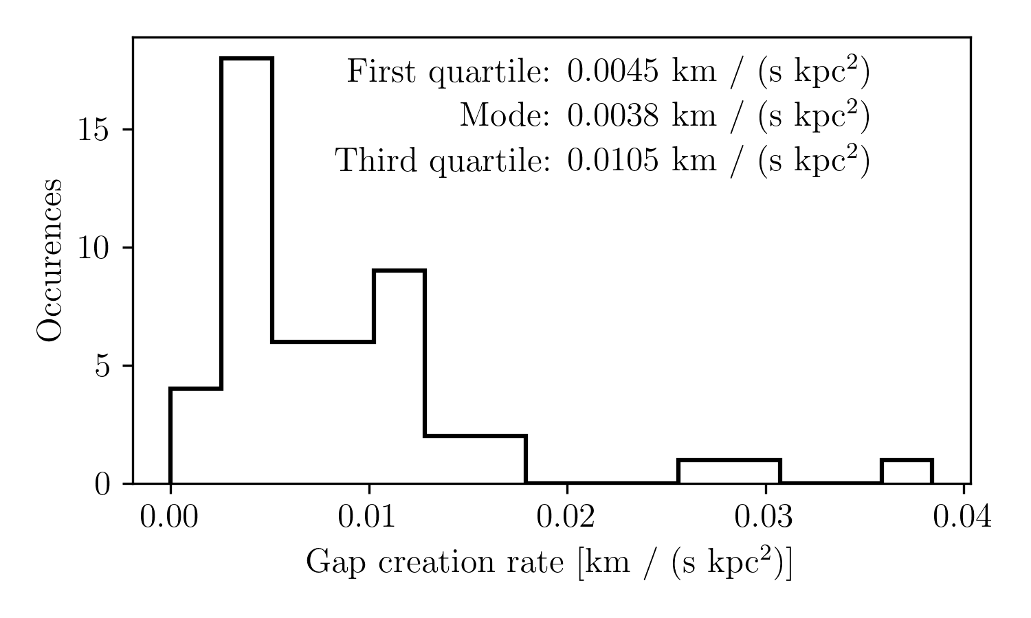
We need a more sophisticated statistic to compare our results to other simulations, so we turn to the gap creation rate developed by Carlberg (2012). The gap creation rate is the number of gaps that appear per unit time and is normalized by the stream’s length. For our simulations, this rate is given by: \[\label{eq:gap_creation_rate} \mathcal{R}_{\mathrm{Pal 5}} = \frac{1}{T}\int_{0}^T l^{-1}(t) \sum_i \delta(t-t_i) dt,\]where \(T\) is the total integration time, \(l(t)\) is the length of the stream, and \(\sum_i \delta(t-t_i)\) sums over the gap occurrences, with \(i\) indexing over the number of gaps in a given simulation. Here, \(\delta\) represents the Dirac delta function. This expression can be simplified to:\[\mathcal{R}_{\mathrm{Pal 5}} = \frac{1}{T} \sum_i \frac{1}{l (t_i)}.\]

This computation allowed us to analyze the distribution of gap creation rates across all simulations. Notice that since the gap creation rate adds in parallel, naturally, gaps that occur at earlier times when the stream was shorter are weighted higher than those that occur when the stream is longer. Fig. 1 presents these results which are is roughly consistent with a simple estimate of the average gap creation rate: with 73 gaps over 5 Gyr of integration time for a stream about 20 kpc in length, the naive estimate is approximately 0.015 km s\(^{-1}\) kpc\(^{-2}\) (which is roughly equivalent to \(0.015~\rm{Gyr^{-1}kpc^{-1}}\)). This naive estimate is about double the weighted mean gap creation rate of 0.009 km s\(^{-1}\) kpc\(^{-2}\) and is higher because it does not account for the growth of the stream over time, unlike Eq. [eq:gap_creation_rate].

Lastly, we note that of the 73 observed gaps, only eight are in the trailing tail, and the rest are in the leading tail, which is a surprising result. A priori, since the star particles escape at similar rates from the L\(_1\) and L\(_2\) Lagrange points, each tail is of similar length and density. The main difference between the two tails is that the leading tail is closer to the Galactic center than the trailing tail by about 400 pc. Since the lengths are equal, and the offset between the tails is slight compared to the Galactocentric distance of about 10 kpc, we expected the gaps in each tail to be more or less the same. We can compute the probability of observing the unequal occurrences through the binomial distribution. First, since the 44 gaps linked to NGC 2808 are the result of the same flyby, they are not independent events. We remove them from this consideration, which leaves 21 gaps in the leading tail and 8 in the trailing. The probability of observing up to 8 successes in 29 trials, given a 50% chance of success, is 1.2%–unlikely, but possible. Additionally, other perturbers impact at consistent times, which may violate the assumption of independent events, as seen with NGC 2808.

Impact geometry and parameters of the perturbers

With the perturbers identified, we perform statistical analysis to understand the conditions necessary for a globular cluster to induce a gap in the Palomar 5 stream. We turn to impact theory, which in its simplest form is presented in works such as Binney and Tremaine (2008). Consider two particles: one stationary and the other moving past it. The impact parameter is the distance between the two particles at the point of their closest approach. The impulse approximation is employed, which assumes that the velocity of the perturber remains unchanged during the interaction. This assumption simplifies the computation.

To understand how the impacted particle is perturbed, one needs to compute its change in momentum, which is determined by integrating the force acting on the particle throughout the interaction. A useful approximation for this change in momentum, per unit mass, is the force at the closest approach multiplied by an estimate of the interaction time: \[\label{eq:change_in_momentum} \Delta p \approx \text{Force} \times \text{interaction time} = \frac{GM}{b^2} \times 2\frac{b}{\delta v} = 2\frac{GM}{b \delta v},\]where \(M\) is the mass of the perturber, \(b\) is the impact parameter, \(\delta v\) is the relative velocity of the perturber with respect to the particle, and \(G\) is the gravitational constant.

This equation asserts that a more massive perturber, passing closer to the particle and moving more slowly, will have a greater impact. It is important to note that the momentum change is inversely proportional to the velocity of the perturber. Note that this contrasts with the intuition from elastic collisions, such as those between billiard balls, where higher velocities result in greater impacts.

Erkal and Belokurov (2015) extended this impact theory from one point mass impacting another to studying how an extended body impacts a stream by quantifying the change in momentum of a given particle as a function of its distance from the point of greatest impact along the stream. Erkal and Belokurov (2015) models their perturber as a Plummer sphere, like in our simulations. Since a stream is not a point but has length and an orientation in space, one needs to consider the parallel and perpendicular components of the velocity to describe the impact fully. Consequently, five parameters determine the change in velocity of a given stream particle: \(M\), \(r_p\), \(b\), \(W_\parallel\), and \(W_\perp\), which are the mass of the perturber, size of the perturber, impact parameter, parallel and perpendicular components of the relative velocity. As detailed in Supplemental Material 6.3, we calculated these parameters for all our full simulations by selecting – for each of them – the strongest five flybys of a perturber with the Palomar 5 stream. Thus, we compute 250 impacts and flag those that give way to gaps.

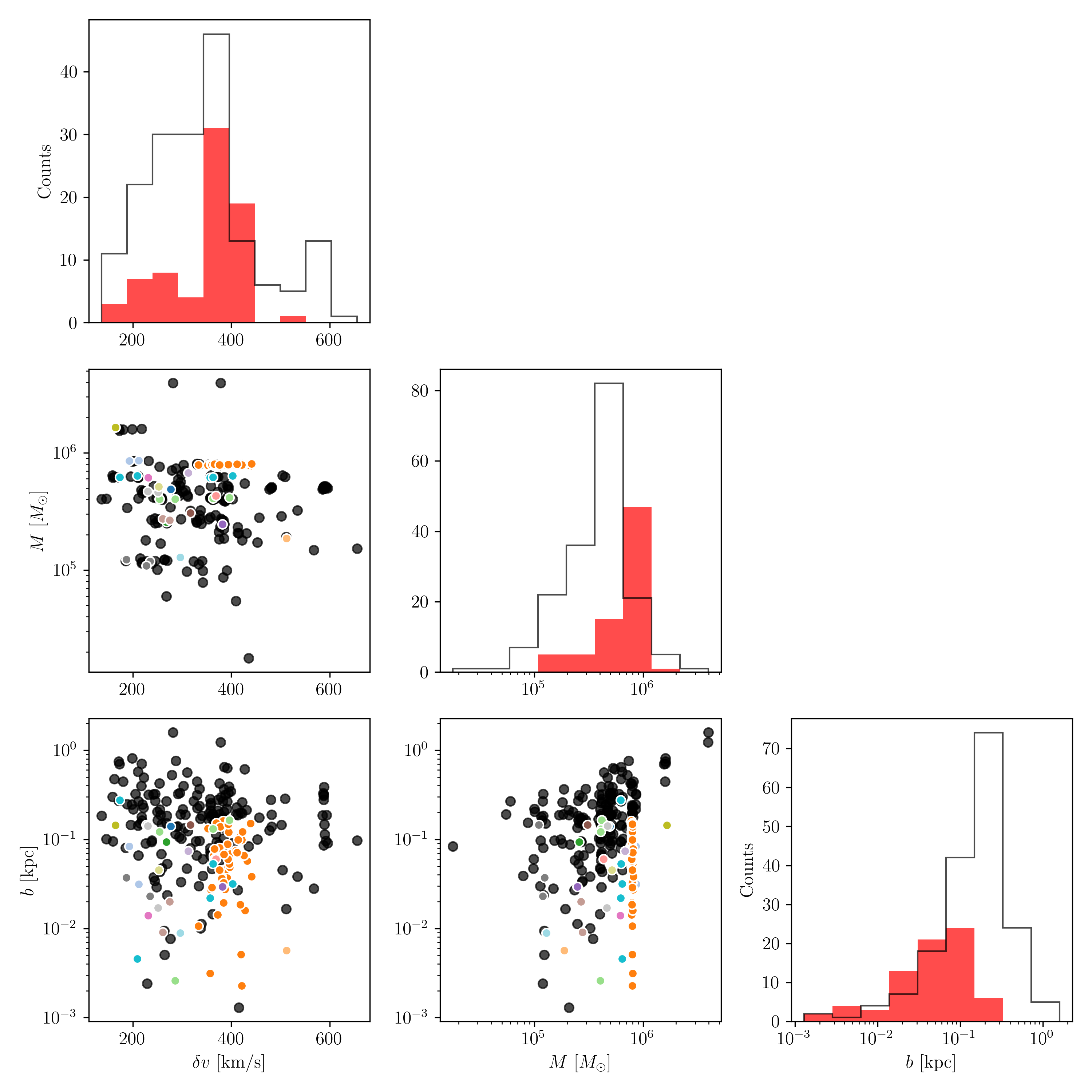
Visual inspection of the five key impact parameters (\(M\), \(r_p\), \(b\), \(W_\parallel\), and \(W_\perp\)) did not reveal a clear distinction between flybys that create gaps and those that do not. Therefore, we only present the quantities from Eq. [eq:change_in_momentum] in Fig. [fig:impact_geometry_statistics].

Note that this figure displays the total relative velocity rather than separating the parallel and perpendicular components, as no specific trends were observed when plotting the two velocity components separately. We also excluded the characteristic cluster radius, which showed little correlation with the results, likely due to the narrow range of globular cluster radii (see Fig. [fig:mass_size_plane]). This factor might be more significant for dark matter subhalos, where size variation is greater.

While Fig. [fig:impact_geometry_statistics] demonstrates that mass, relative velocity, or impact parameter alone cannot predict gap formation, one interesting result emerges: impact parameters greater than 300 pc do not create gaps. The stream widths are roughly 200 pc, as seen in the online appendix. This finding is even more evident when examining the \(b\)-\(M\) plane. A series of perturbers at roughly \(\sim8 \times 10^5 M_\odot\) highlights NGC 2808’s flybys, where all encounters with impact parameters under 200 pc result in gaps, while those beyond this distance do not. In other words, even the most massive globular clusters with masses greater than about \(10^6 M_\odot\) cannot cause gaps if their impact parameters are greater than roughly \(300\) pc. Interestingly, even fast encounters (\(\delta v > 300\) km/s) can produce gaps for impact parameter values below this threshold. Perhaps this is not surprising, since the range of possible relative velocities is much less than that of mass and impact parameters, which vary by two and three orders of magnitude, respectively. In contrast, the relative velocities only vary by about a factor of three.

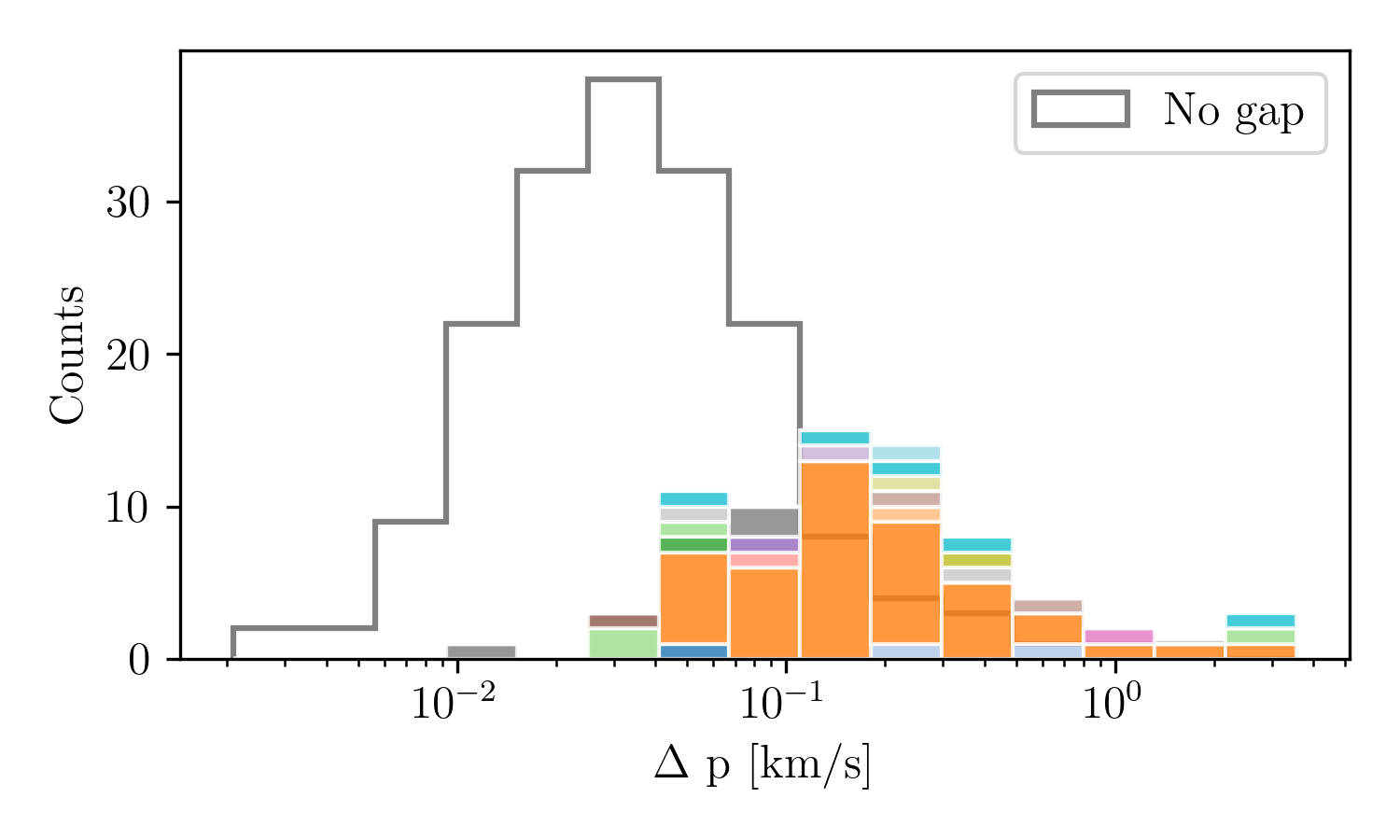
Once all the key impact parameters are estimated, we can use Eq. [eq:change_in_momentum] and calculate \(\Delta p\), the change in momentum (per unit mass) imparted by a cluster flyby on Palomar 5 stream. Fig. 2 shows the distribution of imparted change in momentum for all impacts that produce a gap compared to those that do not. On average, encounters that lead to gap creation impart a change in momentum on stream particles, which is a factor of 10 higher than encounters that do not form gaps (but with some overlap in the low-velocity tail). Interestingly, changes in momentum, which lead to gap creations, extend over a large range in velocities. There is a factor of about 100 between the smallest and largest changes with NGC 2808 (orange color in the histogram) imparting changes in the velocity of stream particles, which redistribute over the whole range of \(\Delta p\).

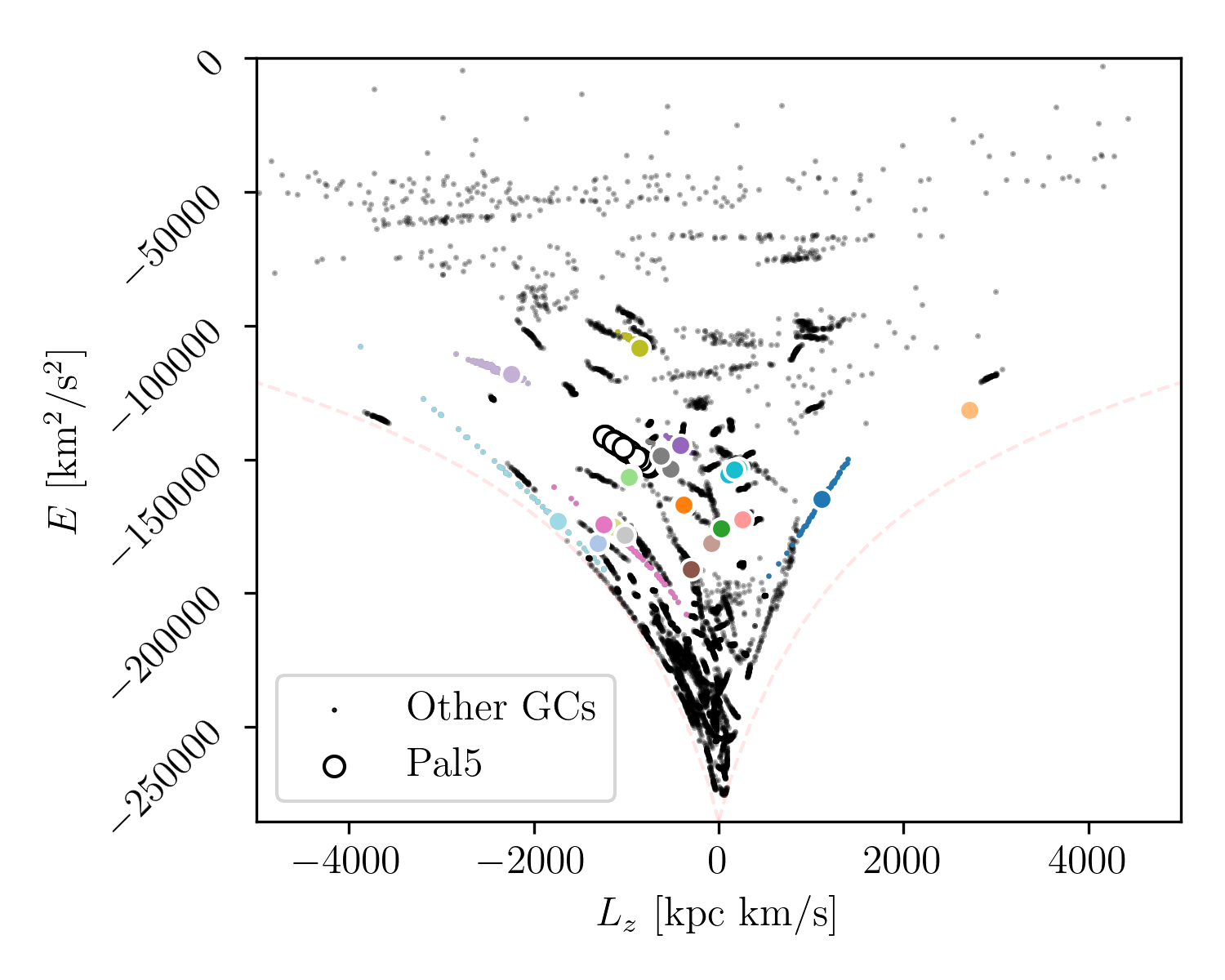
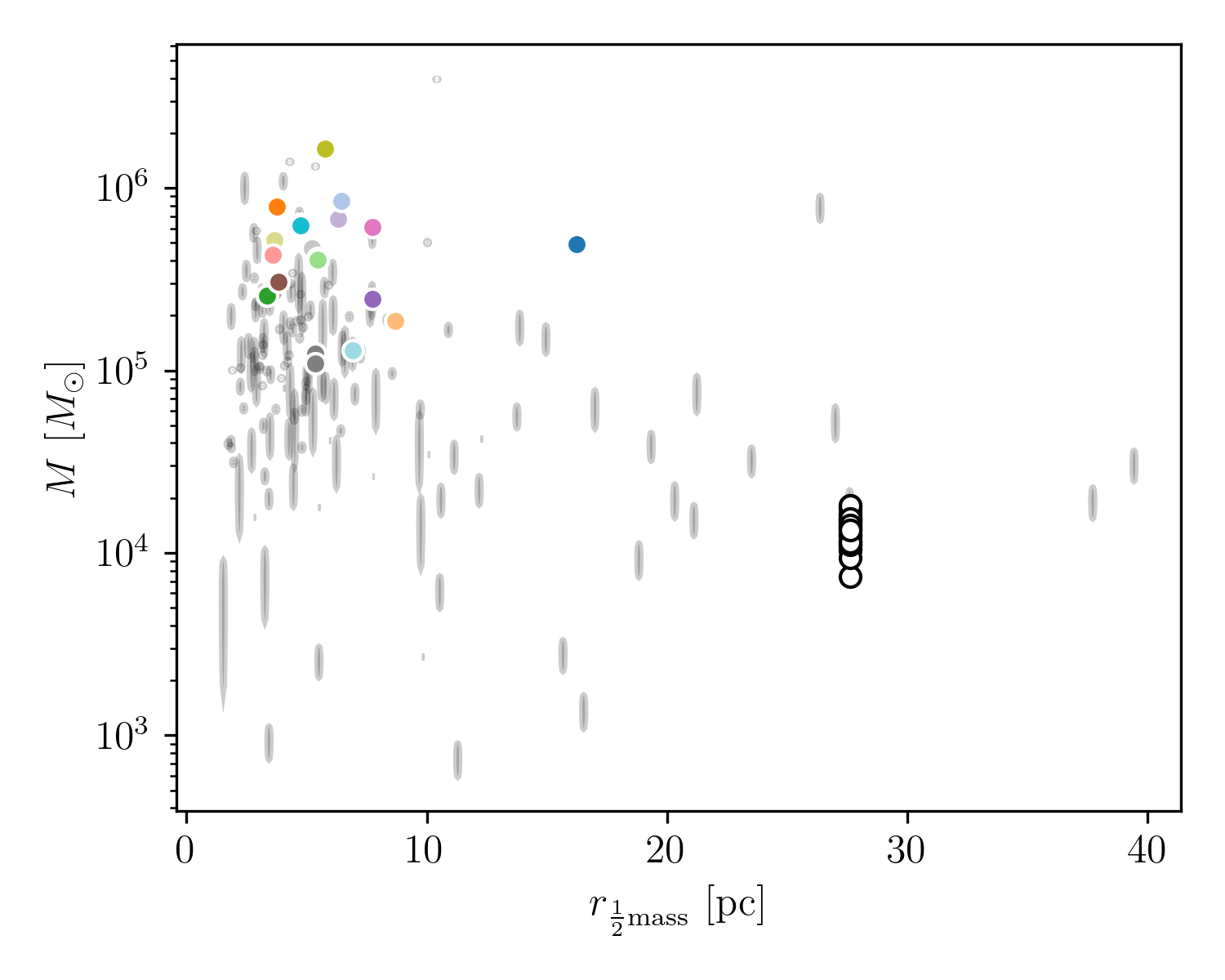
In addition to characterizing the parameters governing cluster encounters with the stream, since we know which clusters have produced gaps on the tail of Palomar 5, we can also verify their orbital and structural properties. Fig [fig:mass_size_plane] shows just this, where we first show the clusters’ mass and size (i.e., half-mass radius) that cause gaps on the tails of Palomar 5, dividing them from those that do not. As can be seen, no cluster with mass below \(10^5 M_\odot\) causes gaps on the Palomar 5 stream, and all perturbers, except FSR 1758, have a half-mass radius below 10 pc. Even more interesting is their distribution in the E-L\(_z\) plane, which shows that the clusters that cause gaps are on both direct and retrograde orbits (negative and positive values of \(L_z\)). However, all of the perturbers exist in an energy interval between \(-2\) and \(-1 \times10^5~\mathrm{km}^2\mathrm{s}^{-2}\), which is because only clusters within Palomar 5’s orbital space can interact with the stream: clusters with higher orbital energies tend to have larger apocenters than that of Palomar 5 and thus spend most of their time away from Palomar 5’s orbital volume.

Finally, it is worth noting the location of impacts with the stream, specifically whether they occur when Palomar 5 is near its pericenter. Fig. [fig:mass_size_plane]’s bottom panel shows that encounters can occur at all orbital phases of Palomar 5, when it is close to the pericenter, but also very far away from it, at the outskirts of its orbital space. However, when taken all together, the location of gap-creating impacts shows a strong negative correlation with the Galactocentric radius \(r\), with the number \(N\) of encounters favorable to gap formation going as \(N = -2.5r + 50\) (with a Pearson coefficient of -0.86). While there are more clusters near the Galactic center, clusters naturally spend more time near their apocenters, and the lower relative velocities in these regions should favor gap creation. However, this result suggests that the cluster Galactic number density outweighs these factors when determining the number of gaps. The results are for Palomar 5 only, and a future study would need to investigate streams along various orbits before generalizing this conclusion.

Comparison to observations

We briefly compare our simulated gaps to the literature on Palomar 5. In the bottom panel of Fig. [fig:decomposition], we compare the tracks of Palomar 5 that were compiled in galstreams by Mateu (2023). The mid-point positions of the streams do not have the same Galactocentric positions as Palomar 5 from Baumgardt’s catalog, and this difference creates an offset when projected into tail coordinates. Moreover, since we sample the distances to Palomar 5, the Galactocentric position within the Baumgardt catalog varies. 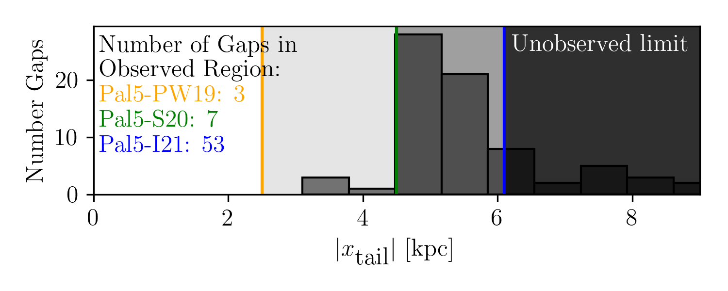To combat this, we position the mid-point of the Galstream tracks at the cluster’s center of mass, allowing us to compare the length of the observed tracks to our simulated streams. We use the three tracks Pal5-PW19, Pal5-S20, and Pal5-I21 from Price-Whelan et al. (2019), Sollima (2020), and R. Ibata et al. (2021), respectively. For each track, we found the distance from the cluster in both directions, counting the number of gaps within this range, and we present this in Fig. 3. In the maximum limit, many gaps could appear at a rate of about one per realization. However, only a few gaps occur at the shortest reported stream length. We note that the gap generated by the recent perturbation induced on the stream by the passage of NGC 2808 (whose occurrence is very likely according to our models) sits in a portion of the simulated tail which is at the edge of the observed one (see bottom panel in Fig. 2). This element and the fact that this gap is skinny, because it is very recent, probably make its detection difficult.

We observe no gaps within 3 kpc of the cluster in our simulation. There may be a few reasons for the absence of gaps in the portion of the tails closer to the cluster center. First, as Sanders, Bovy, and Erkal (2016) demonstrated, the dispersion of action-frequencies in the stream plays a role. For instance, the frequency corresponding to the azimuthal action, \(J_\phi\), is \(\dot\theta_\phi = - \frac{\mathcal{\partial H}}{\partial J_\phi}\) and where \(\theta_\phi\) is the angle describing the position of the particle phase space between momentum (\(p_\phi\)) and position (\(\phi\)) axes—where \(\phi\) is the azimuthal angle between the x-y axes in physical space. Stream regions with well-separated frequencies are more susceptible to gap formation, while those with a wide frequency range (near the cluster) tend to erase the history of impacts. Thus, for a gap to form, the imparted change in frequency must exceed the range of frequencies in the impacted region. Therefore, the strong flybys close to the cluster were inconsequential for gap formation.

Another possible explanation is the different thicknesses of the simulated tails at different distances from the cluster’s center. At distances less than 3 kpc from Palomar 5, the tails are skinny, with a typical thickness of less than 100 pc. To cause gaps in these regions, the clusters would have to pass close to the stream, with impact parameters similar to the thickness itself. We note that the thinness of the tails at these distances is probably a direct consequence of the initial parameters we chose for the simulation. For Palomar 5, 5 Gyr years ago, we assumed the same internal parameters (mass and size) as the cluster today. With such parameters, after 5 Gyr of evolution, our system has lost most of its mass, and therefore, the part of the tails closest to the cluster itself, whose density depends mainly on the most recent mass loss (see, for example, Fig. A.3 in A. Mastrobuono-Battisti et al. 2012), is necessarily very thin because the simulated cluster has essentially no more mass to lose. This last point also has a consequence in the gap creation rate, which we derived at the end of Sect. 3.3: with only 70% of the tail (\(\sim\) 14 kpc over 20 kpc, excluding the innermost \(\pm 3\) kpc from the cluster center) suitable for forming gaps, the gap creation rates are about 50\(\%\) higher than those estimated in the previous section, where values have been derived taking into account the full tail extent. This gap creation rate would still not be high enough to reproduce the number of gaps in Palomar 5’s tails, as reported by Carlberg, Grillmair, and Hetherington (2012). Their study suggested the presence of five gaps with a 99 % detection confidence, leading to a gap creation rate of 0.17 Gyr\(^{-1}\) kpc\(^{-1}\). If correct, this rate would be too high to be explained by Galactic globular clusters only.

An additional explanation for the absence of gaps in the inner regions of a stream is given in App. 6.4. Briefly, the eccentricity of an orbit induces tidal shocking at the pericenter passages that cause episodes of increased mass loss where the escaped stars leave with a higher mean velocity and greater velocity dispersion. In essence, streams from progenitors on eccentric orbits are made of two components: a continuous flow of stars plus many packets of stars that burst out from pericenter passages. The gap impact occurs at a single position, creating a gap in each subpopulation. However, the gaps have different drift rates across the groups, and they eventually go out of phase, erasing the impact’s signature. The packets of stars disperse with time. However, bursts contribute to more escaped stars as the simulation evolves than the continuous outflow. As a result, at late stages of the simulation, the region nearest to the globular cluster is made of distinct yet overlapping populations. After an impact in this location, the impact site between the groups quickly goes out of phase.

Discussion

The simulations presented in this paper suggest that, in the last 5 Gyr of evolution, Palomar 5’s stream could have experienced multiple close encounters with other Galactic globular clusters, some of which can create gaps – even a few kiloparsecs wide – in its tails. Currently, the literature debates whether or not a gap exists in the observed portion of Palomar 5 tails. Rodrigo A. Ibata, Lewis, and Martin (2016) found no statistically significant gap in Palomar 5 tails, while Erkal, Koposov, and Belokurov (2017), analyzing the same dataset as Rodrigo A. Ibata, Lewis, and Martin (2016), suggested the presence of a few dips and gaps in the tails, at angular distances between \(2^\circ\) and \(9^\circ\) from the cluster center (see also Bonaca, Pearson, et al. 2020). While our simulations produced 73 gaps across 50 realizations, only about 22 are beyond the current length of the observed portion of the stream, which means, on average, we obtain at least one gap from a globular cluster within the past 5 Gyr. However, we did not attempt to create mock observations or simulate a full detection process accounting for the challenges of disentangling field stars from stream stars. While such an analysis would be valuable, it is beyond the scope of this study.

Our simulations produce a stream for Palomar 5 that is longer than the currently observed extent. In simulations, stream detections are straightforward because we can use reference runs to clearly separate stream particles from the field and compare against a known “true” structure. In contrast, observational data are inherently more challenging due to magnitude limits, contamination from field stars, and the lack of a ground truth for comparison.

The factors mentioned above could lead one to conclude that the number of gaps identified in this study could represent an upper limit. However, this conclusion is incomplete. Globular clusters lose mass and evaporate over time, leading to an incomplete catalog of perturbers. Moreover, the present-day masses used in our simulations are likely lower than the historical masses of these clusters. For example, Pearson et al. (2024) conducted a study simulating the dissolution of a realistic globular cluster population to identify how many stellar streams we should expect in the Milky Way and used a mock catalog of globular clusters with masses above 10\(^4 M_\odot\) totaling about 10,000 clusters. Their setup implies that more perturbers could have been present in the past, potentially increasing the frequency and number of gaps in Palomar 5’s stream.

We note that our results seem to be in tension with the conclusions of Banik and Bovy (2019), who presented a numerical study of Palomar 5 tails, orbiting a Milky Way-like potential, where both dark matter subhalos and baryonic sub-structures (Galactic bar, spiral arms, giant molecular clouds, globular clusters) were taken into account to quantify the importance of these latter in density variations in Pal5 streams. While their methods are extremely similar to ours, their analysis diverges significantly. Specifically, Banik and Bovy (2019) focused on examining power spectra, analyzing variations in the one-dimensional stream density in stellar counts along the length of the stream. Upon comparison with our simulations, we observe that the power spectra from our full simulations that include globular clusters and the reference simulations that do not significantly differ. We suggest that this may be due to the signal from only one or two gaps caused by globular clusters not being sufficient to produce notable differences in the overall power spectrum. Additionally, Banik and Bovy (2019) may not have inspected the profiles for individual gaps, which may be why they did not report them. Further investigations would be needed to confirm this interpretation and thoroughly assess the impact of globular clusters on stream density profiles.
Erkal, Koposov, and Belokurov (2017) also present a study about the impact of globular clusters in producing gaps on the Pal 5 stream. In section 6.3 of their article, Erkal, Koposov, and Belokurov (2017) discuss the fact that globular clusters with masses greater than \(10^6~\textrm{M}_\odot\) are rare in the Galaxy, especially at distances compatible with the orbit of Pal 5, while – based on previous works – they estimate that subhalos of dark matter of similar mass are at least three times greater in number. This difference leads them to conclude that the gaps they report in the Pal 5 streams are more likely to be induced by dark matter subhalos than by globular clusters.

However, as we show in this paper, even clusters with masses below \(10^6~\textrm{M}\odot\) can produce gaps. The clusters perturbing the Pal 5 stream are clusters with masses up to 10 times lower than those considered by Erkal, Koposov, and Belokurov (2017). It is thus possible that Erkal, Koposov, and Belokurov (2017) have underestimated the impact of globular clusters’ close passages on a stream such as Pal 5. It is more difficult, however, to make a comparative analysis between the role of clusters and subhalos at equal stellar mass. Being less dense than globular clusters, subhalos should produce less intense perturbations on streams (for fixed impact parameters and relative velocities). We can derive from Sanders, Bovy, and Erkal (2016)’s third figure that a more concentrated system delivers a higher velocity kick but over a shorter distance, while a more spread out system will affect more stars yet perturb them less. A systematic comparative analysis to quantify the role of clusters and subhalos in producing gaps and perturbations in stellar streams still needs to be done.

The impact of globular clusters’ close interactions with stellar streams has also been the object of another recent paper by Doke and Hattori (2022), who concluded that the chance for GD-1 gaps, which have been reported in several works (see, for example, Bonaca et al. 2019; T. J. L. de Boer et al. 2018; T. de Boer, Gieles, and Erkal 2020) to be produced by globular clusters is very low. This result is not necessarily in contradiction with ours since GD-1 has a pericenter which is almost twice that of Palomar 5 (see, for example Malhan and Ibata 2019). As discussed in Sect. 3.3, the number, \(N\), of close encounters that lead to gap creation is anti-correlated with the distance \(r\) to the Galactic center. If we naively use the same radial dependence of gaps from Palomar 5 for GD-1 by swapping a pericenter from 6 kpc to 16 kpc, we would reduce the number of gap-favorable impacts by more than a factor of 2. Moreover, we note that Doke and Hattori (2022) pre-selects the globular clusters that could have experienced a close encounter with the GD-1 stream by selecting only clusters that pass at a distance of less than 0.5 kpc from the stream, having a relative velocity smaller than 300 km/s. As shown in our Fig. [fig:impact_geometry_statistics], bottom-left panel, in the case of Palomar 5, this choice would lead to excluding most of the encounters favorable to gap creation, which turn out to have relative velocities above 300 km/s, reducing the total to just 19 gaps. It would be interesting to repeat a similar study as the one made by Doke and Hattori (2022) for GD-1, imposing no selection on possible candidate clusters.
As already suggested in previous works which have studied the impact of baryonic structures on Palomar 5 tails (Pearson, Price-Whelan, and Johnston 2017; Banik and Bovy 2019), this cluster may lie in a region of the phase-space which is not favorable to distinguish gaps created by dark matter subhalos from gaps created by baryonic structures, such as the Galactic bar and giant molecular clouds. Our study shows that close encounters with globular clusters constitute a further element that confuses a simple interpretation of the observed Palomar 5 stream gaps (if any). Other clusters and streams in the orbital energy range of Palomar 5 may suffer from the same difficulty. Going to lower orbital energies worsens the situation because the effect of the Galactic bar, giant molecular clouds, and interactions with globular clusters becomes even more efficient. In the innermost regions of the Galaxy, where the density of dark matter subhalos is maximal, globular cluster streams are intrinsically more difficult to find, in addition to the fact that the dynamical times in these regions become so small that the stars lost from globular clusters do not redistribute themselves for the most part into thin structures (see Ferrone et al. 2023). It is thus probably only at larger distances from the Galactic center than those spanned by Palomar 5’s orbit that the impact of dark matter subhalos may become dominant, but one should bear in mind that at these distances, the number density of subhalos also decreases. In the future, it will be interesting to apply the type of study conducted here to the whole set of streams to quantify the regime in which they are favorable to the creation of gaps from baryonic structures.

Conclusions

Our study demonstrates that globular cluster flybys can produce density gaps in the stellar streams of Palomar 5. The occurrence and characteristics of these gaps depend on the stream’s dynamical and structural properties, the perturber’s mass, and the impact parameter. While our simulations predict the formation of gaps in Palomar 5’s tails, the predicted gaps do not align with the regions of the stream currently observed. Several factors contribute to the absence of simulated gaps in the observed portions of Palomar 5’s tails, including the stream’s varying thickness, the dispersion of action frequencies near the cluster, and the initial conditions adopted in our simulations.

The broader implications of our findings indicate that globular cluster interactions add a layer of complexity to interpreting stellar stream substructures, complicating efforts to distinguish between baryonic and dark matter-induced gaps. While Palomar 5’s phase-space region may not be ideal for isolating the impact of dark matter subhalos, extending this analysis to other streams, particularly those at larger Galactocentric distances, could provide clearer insights.

Future work should involve a systematic comparison of gap creation rates across various Galactic potentials and extend the scope to a wider range of streams and globular clusters. Such a work could disentangle regimes where baryonic and dark matter-induced substructures can dominate gap creation, shedding light on the elusive influence of dark matter subhalos on stellar streams. Additionally, we can continue to add realistic physics to the Galactic environment, such as the merger of the Sagittarius dwarf galaxy, the passages of the Large and Small Magellanic clouds, as well as a time-evolving globular cluster population that compensates for the clusters’ mass loss, evaporation, and similarly add members from the current incomplete census.

Supplementary Material

Gap detection

For each of the 50 simulations, we compare the final snapshots between the reference and full simulations using the tail coordinate system, as shown in Fig. 4. We only saved the reference simulations at the final time stamps, thus from Eq. [eq:data_volume_estimate] where \(N_{ts}\)=1, leading to a data volume of about one hundred measly megabytes. We inspected these differences by generating 2D density maps of the streams. Additionally, we marginalized over the \(y'\)-coordinate to produce 1D density profiles along the \(x'\)-axis. We show these comparisons in the results section (see Fig. [fig:profiles]).

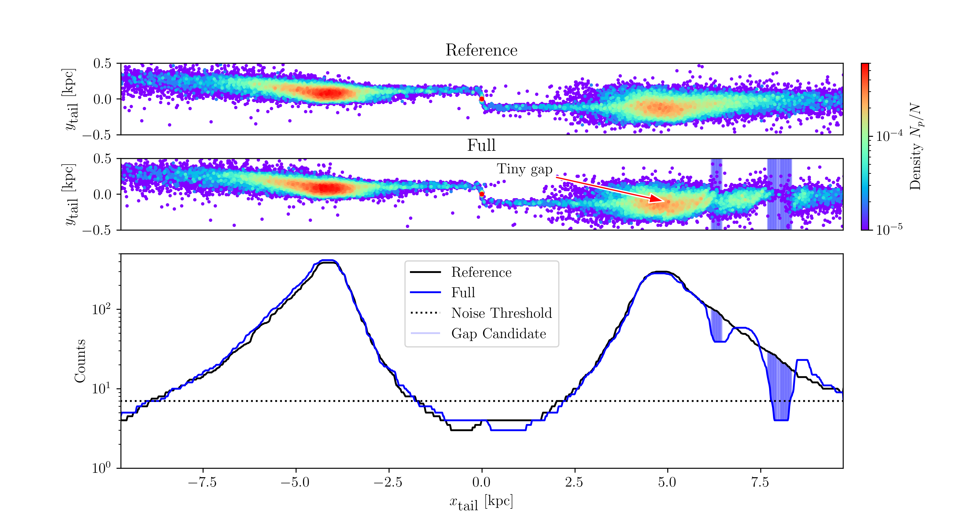
To construct the 1D density profiles, we binned the data using the \(\sqrt{N}\) rule, where \(N\) is the number of data points (\(N_p = 10^5\)). After binning the 1D profiles, we apply a median boxcar smoothing technique. At each bin, we select a number of adjacent data points from both sides, place them in a list, and replace the central value of the bin with the median. We use 10 adjacent points per side, corresponding to a smoothing length of approximately 1 kpc. This procedure reduces high-frequency noise and smooths the profiles. For instance, notice the absence of a high mass peak indicating the center of mass in the bottom panel of Fig. [fig:profiles].

With the smoothed 1D density profiles in hand, we search regions where the full simulations are significantly underdense compared to reference simulations, surpassing stochastic fluctuations. We first impose a signal-to-noise ratio threshold, \(\mathcal{SNR}\). The signal is the log of the counts per bin from the reference 1D density profile; we propagate errors assuming a Poisson distribution. We then compute a threshold for the number of counts in the reference simulation, \(N_v\), using the transcendental equation: \[\mathcal{SNR} = \ln(10) \log_{10}\left(N_v\right) \sqrt{N_v}.\] By setting \(\mathcal{SNR} = 5\), we solve for \(N\) using scipy.optimize.fsolve, finding that \(N\) must be greater than 7. After discarding insignificant bins (i.e., those with counts below the threshold), we computed the log ratio of the counts between the reference and full simulations: \[\mathcal{R}_i = \log_{10}\left(\frac{N_{f,i}}{N_{v,i}}\right),\] where \(\mathcal{R}_i\) is the log ratio, \(N_{f,i}\) are the counts from the full simulation, and \(N_{v,i}\) are the counts from the reference simulation for each bin \(i\). We then analyze the \(\mathcal{R}_i\) distribution. If the differences between the density profiles are primarily due to stochastic processes of similar magnitude, this distribution should resemble a Gaussian, as expected from the central limit theorem. Thus, we flag all regions where the density is underdense by more than two standard deviations, which should highlight regions whose underdensity is unlikely to be the result of the sum of stochastic processes but rather the passage of another globular cluster.

However, this method has its limitations, especially when detecting smaller gaps. As outlined by Erkal and Belokurov (2015), since gap growth is a dispersion phenomenon, a small gap is not indicative of a weak impact but a recent one. Additionally, since our streams have finite width, some gaps are oblique with respect to the stream axis. In such cases, marginalizing over \(y'\) erases the gap’s signal, making it impossible to detect in a 1D profile. This limitation is particularly evident in gaps caused by NGC 2808, as discussed in the results. Therefore, this quantitative analysis serves as an aid to visual inspection rather than a complete substitute for it. This method helps with significant, subtle gaps that the eye does not notice in the 2D maps. The online appendix presents these profiles.

Perturber identification

We aim to identify the origin of the gaps observed at the end of the simulation. To this end, we examine the evolution of stream density over time. Instead of using the x’-coordinate, we introduce \(\tau\), which represents time rather than distance. Specifically, \(\tau\) indicates how long a cluster will take to reach a given point in its orbit or how long ago it passed. This choice of coordinates is advantageous because the growth of the stream is approximately linear in \(\tau\). In contrast, in physical space, streams on eccentric orbits expand and contract depending on the orbital phase.

Sanders, Bovy, and Erkal (2016) extended the analysis of Erkal and Belokurov (2015), demonstrating that action-angle variables provide a useful coordinate system for analyzing stream evolution, as actions are conserved quantities and their associated angles grow linearly over time. Although we became aware of this work only after completing our analysis, we note that \(\tau\) is a suitable approximation and behaves similarly to the angle variable corresponding to the azimuthal action: \(\tau \approx \theta_{\phi, i} - \theta_{\phi,\text{GC}}\).

The core of our analysis is presented in Fig. [fig:force-on-orbit]. The bottom panel shows the evolution of the stream density over time. To avoid extremely low-density regions at the stream’s edges, we applied the same density threshold as from Eq. [eq:density_threshold] to focus on the more significant areas of the stream. Next, we modeled Palomar 5’s orbit as a proxy for its stream and sampled points along the orbit to measure the gravitational force exerted by other globular clusters. The top panel of Fig. [fig:force-on-orbit] shows how the total gravitational acceleration on Palomar 5’s stream evolves over its length throughout the simulation.

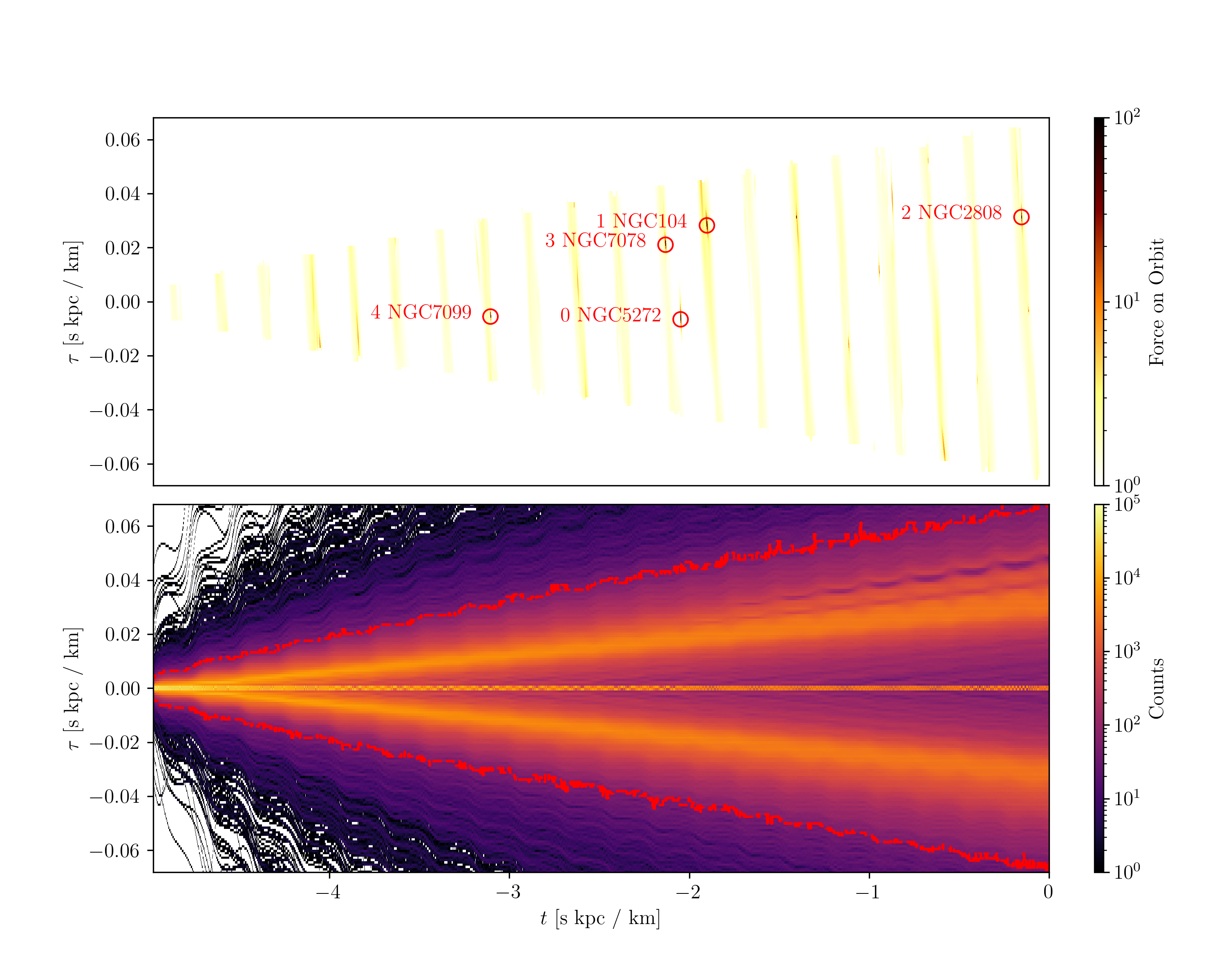
We then used scipy’s ndimage (Virtanen et al. 2020) package to identify the top five local maxima in the data space of gravitational acceleration \(\vec{g}\) as a function of time \(t\) and the stream coordinate \(\tau\). First, we smooth the data space by taking a 5-point moving average kernel. Secondly, we use a maximum filter to locate coordinates in the (\(t,\tau\)) data plane that are local maxima to at least 10 adjacent data points. We order these locations and save the top five strongest interactions. Then, we iterated over the contributions of individual globular clusters to determine which cluster contributed the most to each peak in \(\vec{g}\). We label each significant peak with the corresponding globular cluster.

Afterward, we cross-referenced these peaks with the locations of the gaps identified by studying the density maps and profiles from Fig. [fig:profiles]. The impact leaves a low-density wake in the (\(t,\tau\)) plane for large gaps resulting from strong interactions. the bottom panel of Fig. [fig:force-on-orbit] shows the wakes corresponding to the impacts of NGC 104 and NGC 7808.

Fig. [fig:force-on-orbit] contains some interesting information. Notice the periodic ribbons of force in the \((t,\tau)\) plane. The ribbons are due to pericenter passages where Palomar 5 is getting closer to the center of mass of the globular cluster system. Additionally, for the impacts of NGC 104 and NGC 7078, wakes can be observed in the density map. Another important aspect is that the strongest peak in gravitational force does not necessarily create a gap. Notice how NGC 5272, which was labeled with 0 to indicate that it has the greatest local maxima, does not have a gap. The reason for this is manifold. For instance, the force needs to be modulated with time since the change in momentum is the determining factor and not the peak magnitude of the force. Additionally, there is an offset of about 200 pc between the stream and the orbit, as seen when viewing the stream in tail coordinates, so peaks upon the orbit are good proxies for the stream but are not definitive. We found that the top five greatest impacts accounted for all gaps, except for Sampling 014 as shown in Fig. 3 of our extended list of figures, whose gap from NGC 6584 corresponded to the 7th peak.

We compile the results of this analysis into a table. Each row of the table corresponds to a gap; its corresponding suspects are the columns. The culprit is labeled as TRUE. For a handful of simulations, to double-check that we make the correct verdict, we recompute the simulations, yet individually adding one globular cluster at a time. As a result, we can confirm that singular gaps arise from the suspected clusters. Fig. [fig:decomposition] shows one such example.

Reconstruction of the impact geometry

As discussed in Sect 3.3, five parameters determine the change in velocity of a given stream particle: \(M\), \(r_p\), \(b\), \(W_\parallel\), and \(W_\perp\). In the following, we describe how we estimated these parameters during impacts in our simulations.

To achieve this, we identify the impact of the most significant clusters, as determined in the previous analysis in Sec. 6.2. Then, we refine these estimates to pinpoint the exact location of the impact along the stream and the precise moment it occurred. To do so, we fit a third-order parametric polynomial to the stream using the saved snapshots from our simulations:

\[\vec{s}(\tau) = \left\{ \begin{aligned} x(\tau) &= a_0 + a_1 \tau + a_2 \tau^2 + a_3 \tau^3 \\ y(\tau) &= b_0 + b_1 \tau + b_2 \tau^2 + b_3 \tau^3 \\ z(\tau) &= c_0 + c_1 \tau + c_2 \tau^2 + c_3 \tau^3, \end{aligned} \right.\] where \(x\), \(y\), and \(z\) represent the parametric line describing the stream in Galactocentric coordinates, \(\tau\) is the stream coordinate in time as described in the Supplemental Material 6.2, and is used as the independent variable to parameterize the position along the stream. The coefficients \(a_i\), \(b_i\), and \(c_i\) are the polynomial coefficients. We found that a second-order polynomial was insufficient to capture the curvature along the full length of the stream, with divergence at the ends of the tails. A third-order polynomial was sufficient and desirable, as the lowest order adequately captures the stream’s path over the entire length under consideration.

In this analysis, we only consider one side of the stream. For instance, if the impact candidate was in the leading tail, only the star particles with \(\tau > 0\) are used to constrain the stream track. The polynomial coefficients were determined through a minimization method using the Nelder-Mead algorithm from scipy’s optimization package.

Since we saved the simulation snapshots at a temporal resolution of 1 Myr–rather than at the integration time-step, which would have generated excessive data, we must interpolate between snapshots to more precisely estimate the impact geometry. We fit the stream’s shape with a parametric third-order polynomial at the five time steps surrounding the approximate impact time. This time is a period of 5 Myr, sufficiently covering the interaction time. The interaction time can be estimated as \(t \approx \frac{100~\text{pc}}{300~\frac{\text{km}}{\text{s}}} \approx 0.3~\text{Myr}\).

Then, we used a cubic spline interpolation for the coefficients describing the stream’s shape, which allows us to describe each polynomial coefficient as a function of time. Consequently, we can parameterize the stream as a function of both simulation time and position along the stream: \[\vec{s}(t,\tau) = \left\{ \begin{aligned} x(t,\tau) &= a_0(t) + a_1(t)\tau + a_2(t) \tau^2 + a_3(t)\tau^3 \\ y(t,\tau) &= b_0(t) + b_1(t)\tau + b_2(t) \tau^2 + b_3(t)\tau^3 \\ z(t,\tau) &= c_0(t) + c_1(t)\tau + c_2(t) \tau^2 + c_3(t)\tau^3. \end{aligned} \right.\]

The values of the coefficients as a function of time are obtained through linear interpolation, ensuring that the coefficients at the snapshot times match the values constrained by the simulation data.

Next, we fit the trajectory of the perturber with a second-order polynomial. With equations for both the stream and the perturber as functions of time, we identify the time and location of impact by minimizing a cost function, defined as the distance between the stream and the perturber: \[b(t, \tau) = \left\lVert \vec{s}(t, \tau) - \vec{p}(t) \right\rVert,\] where \(\vec{s}(t, \tau)\) is the Galactocentric position of a point on the stream, \(\vec{p}(t)\) is the position of the perturber, and \(b\) is the distance between the two. The minimum value of \(b\), denoted as \(\text{min}(b)\), represents the impact parameter. We performed the minimization using scipy’s optimization package with the L-BFGS-B method, which allowed us to place bounds on \(t\) and \(\tau\), ensuring no extrapolation occurs (Davidon 1991).

Once this minimization is done, determining the relative velocity becomes straightforward. Since the minimization provides the impact parameter, time of impact, and the corresponding value of \(\tau\), we can compute the derivatives of the parametric equations at \(t_{\text{min}}\) and \(\tau_{\text{min}}\). The parallel and perpendicular components of the perturber’s velocity relative to the stream are given by:

\[\begin{aligned} \delta \vec{v} &=\vec{v_p} - \vec{v_s}, \\ w_\parallel &= \left(\delta \vec{v}\right)\cdot \hat{v_s},\\ w_\perp &= \sqrt{\Delta v ^2 - w_\parallel ^ 2}, \end{aligned}\] where \(\vec{v}_p\) and \(\vec{v}_s\) are the velocities of the perturber and the stream, respectively. We compute the strongest five flybys for each of the 50 simulations. Thus, we created a sample of 250 impacts and flagged those that give rise to gaps. We refer the reader to Sect. 3.3 for the presentation and discussion of the results.

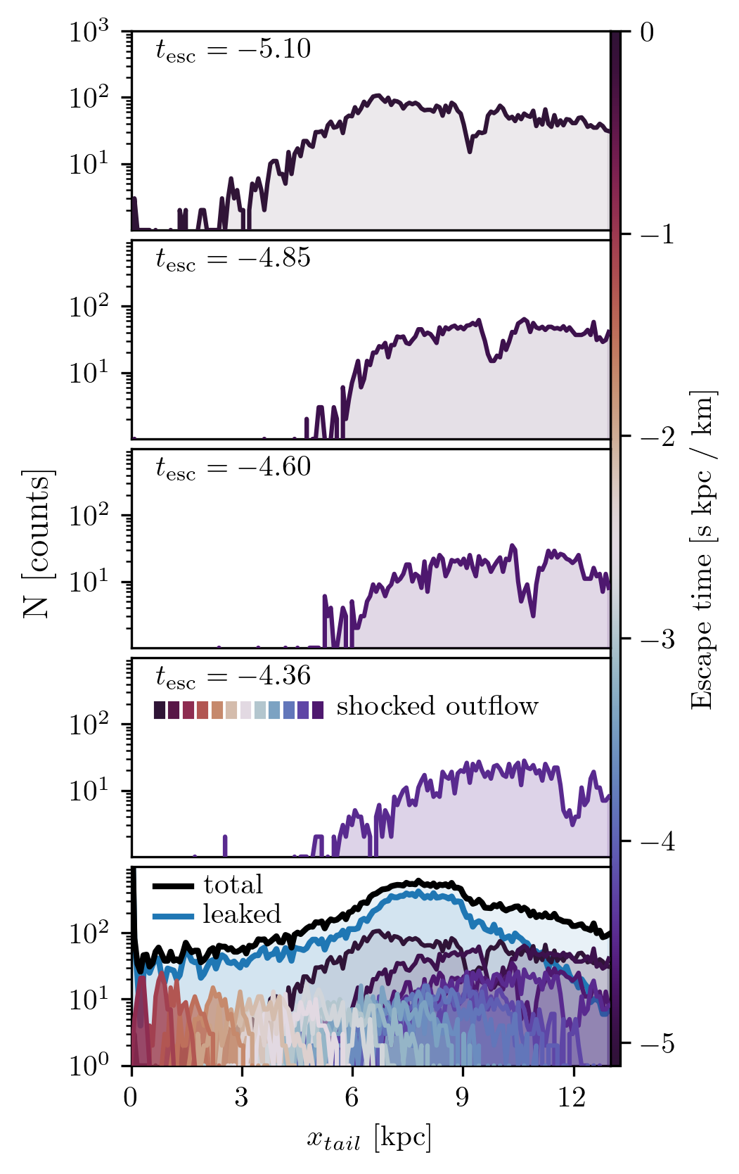
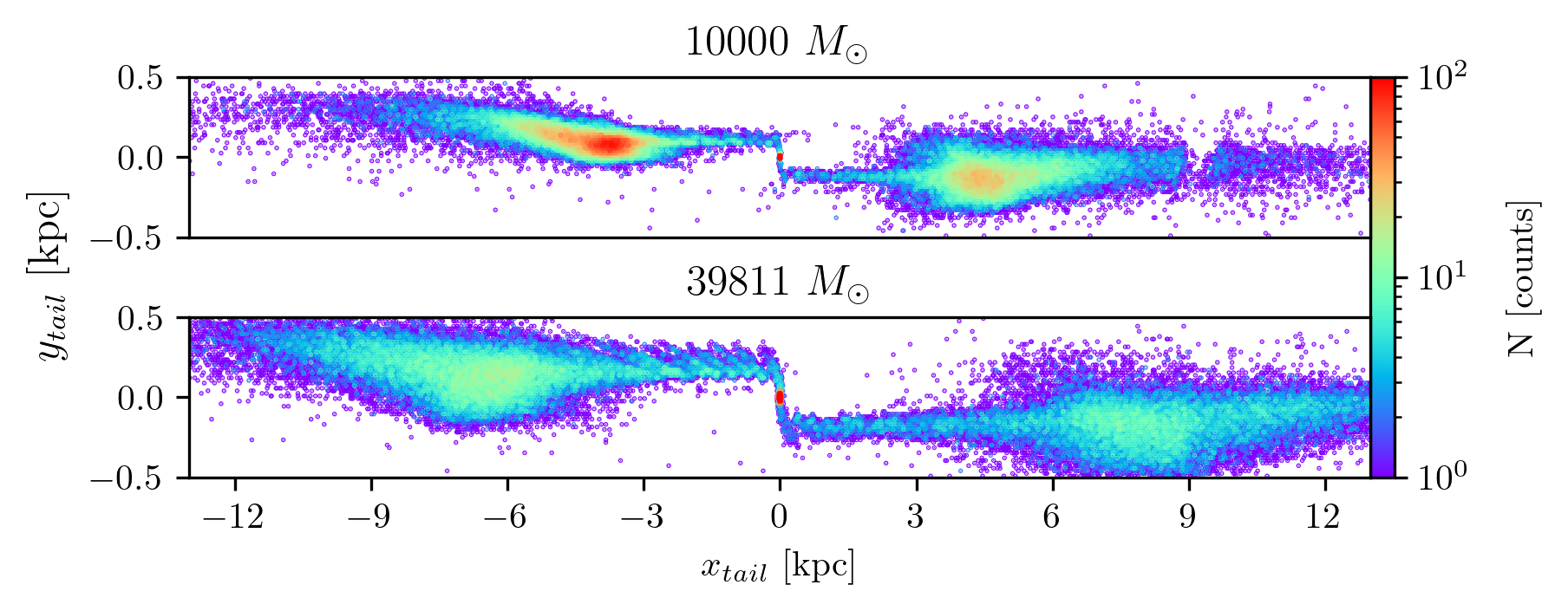
Survival of gaps in streams emerging from more massive globular clusters

In Section 2.2, we emphasized that the conditions chosen to simulate the formation and evolution of streams around Pal 5 are probably unrealistic. By choosing, as we did, the same values for the mass and size of the cluster 5 billion years ago as the cluster has today, we did not take into account the loss of mass and internal evolution of the cluster over time. In particular, the velocity dispersion of the stars in a cluster and the velocity dispersion of the stars leaving the cluster and entering the stream depend on the cluster’s mass. It is therefore legitimate to ask whether, using a progenitor with a different mass and/or size, the gaps survive and whether, in particular, gaps formed several billion years ago can still be visible today.

While we anticipate that a specific study on this aspect is in preparation (Ferrone et al., in prep), we would like to preview a few results here, particularly regarding the gap decoherence phenomenon presented in Fig. 5. First, Fig. [fig:gap_no_more] shows two streams with the same orbital parameters that were impacted by NGC 7078. The top panel shows a stream originating from a host mass of \(10,000\) \(M_\odot\), while in the second panel we increased the mass to \(\sim40,000\) \(M_\odot\). For simplicity, both clusters have the same half-mass radius of 27 pc. The encounter occurred about two and a half billion years ago with NGC 7078, which has a mass of \(5.16\times10^{5}~M_\odot\). The gap persists for the lighter host, yet is barely visible in the case of the more massive host.

Fig. 5 dissects the more massive stream of Fig. [fig:gap_no_more] and explains why the gap does not persist. The bottom panel shows the total density distribution, decomposed into two profiles: stars that are either leaked or shocked out of the cluster. By shocked, we mean stars that are lost during pericenter passages. Tidal forces generally scale with \(r^{-3}\), and thus significantly intensify during pericenter passages (see Fig. 3 of Dehnen et al. (2004) for an illustration of the magnitude of tidal forces along an orbit). A consequence of these passages is that many more stars escape, fleeing with higher mean velocity and velocity dispersion—this can be visualized in the “Christmas tree” illustration in Fig. A.3 of A. Mastrobuono-Battisti et al. (2012). We consider the continuous outflow of stars between pericenter passages to be leaked stars. We identify pericenter passages by computing each local minimum of the cluster’s Galactocentric 3D radius using scipy.signal.find_peaks. The duration of each shock is given by \(t_{\textrm{shock}} = 2\sqrt{r/|\nabla\Phi|}\), where \(r\) is the Galactocentric radius and \(|\nabla\Phi|\) is the magnitude of the acceleration from the Galactic potential. Stars within this time range around a given pericenter passage are all given the same color and shown as individual groups in the first through fourth panels of Fig. 5.

Amorisco, Nicola C. 2021. “Cold dark matter subhaloes at arbitrarily low masses.” arXiv e-Prints, November, arXiv:2111.01148. https://doi.org/10.48550/arXiv.2111.01148.

Amorisco, Nicola C., Facundo A. Gómez, Simona Vegetti, and Simon D. M. White. 2016. “Gaps in globular cluster streams: giant molecular clouds can cause them too” 463 (1): L17–21. https://doi.org/10.1093/mnrasl/slw148.

Astropy Collaboration, Thomas P. Robitaille, Erik J. Tollerud, Perry Greenfield, Michael Droettboom, Erik Bray, Tom Aldcroft, et al. 2013. “Astropy: A community Python package for astronomy” 558 (October):A33. https://doi.org/10.1051/0004-6361/201322068.

Banik, Nilanjan, and Jo Bovy. 2019. “Effects of baryonic and dark matter substructure on the Pal 5 stream” 484 (2): 2009–20. https://doi.org/10.1093/mnras/stz142.

Banik, Nilanjan, Jo Bovy, Gianfranco Bertone, Denis Erkal, and T. J. L. de Boer. 2021. “Novel constraints on the particle nature of dark matter from stellar streams” 2021 (10): 043. https://doi.org/10.1088/1475-7516/2021/10/043.

Baumgardt, H., and M. Hilker. 2018. “A catalogue of masses, structural parameters, and velocity dispersion profiles of 112 Milky Way globular clusters” 478 (2): 1520–57. https://doi.org/10.1093/mnras/sty1057.

Baumgardt, H., M. Hilker, A. Sollima, and A. Bellini. 2019. “Mean proper motions, space orbits, and velocity dispersion profiles of Galactic globular clusters derived from Gaia DR2 data” 482 (4): 5138–55. https://doi.org/10.1093/mnras/sty2997.

Baumgardt, H., A. Sollima, and M. Hilker. 2020. “Absolute V-band magnitudes and mass-to-light ratios of Galactic globular clusters” 37 (November):e046. https://doi.org/10.1017/pasa.2020.38.

Baumgardt, H., and E. Vasiliev. 2021. “Accurate distances to Galactic globular clusters through a combination of Gaia EDR3, HST, and literature data” 505 (4): 5957–77. https://doi.org/10.1093/mnras/stab1474.

Belokurov, V., N. W. Evans, M. J. Irwin, P. C. Hewett, and M. I. Wilkinson. 2006. “The Discovery of Tidal Tails around the Globular Cluster NGC 5466” 637 (1): L29–32. https://doi.org/10.1086/500362.

Bernard, E. J., A. M. N. Ferguson, E. F. Schlafly, M. Abbas, E. F. Bell, N. R. Deacon, N. F. Martin, et al. 2014. “Serendipitous discovery of a thin stellar stream near the Galactic bulge in the Pan-STARRS1 3\(\pi\) Survey.” 443 (September):L84–88. https://doi.org/10.1093/mnrasl/slu089.

Bernard, Edouard J., Annette M. N. Ferguson, Edward F. Schlafly, Nicolas F. Martin, Hans-Walter Rix, Eric F. Bell, Douglas P. Finkbeiner, et al. 2016. “A Synoptic Map of Halo Substructures from the Pan-STARRS1 3\(\pi\) Survey” 463 (2): 1759–68. https://doi.org/10.1093/mnras/stw2134.

Binney, James, and Scott Tremaine. 2008. Galactic Dynamics: Second Edition.

Bonaca, Ana, Charlie Conroy, David W. Hogg, Phillip A. Cargile, Nelson Caldwell, Rohan P. Naidu, Adrian M. Price-Whelan, Joshua S. Speagle, and Benjamin D. Johnson. 2020. “High-resolution Spectroscopy of the GD-1 Stellar Stream Localizes the Perturber near the Orbital Plane of Sagittarius” 892 (2): L37. https://doi.org/10.3847/2041-8213/ab800c.

Bonaca, Ana, Marla Geha, and Nitya Kallivayalil. 2012. “A Cold Milky Way Stellar Stream in the Direction of Triangulum” 760 (1): L6. https://doi.org/10.1088/2041-8205/760/1/L6.

Bonaca, Ana, and David W. Hogg. 2018. “The Information Content in Cold Stellar Streams” 867 (2): 101. https://doi.org/10.3847/1538-4357/aae4da.

Bonaca, Ana, David W. Hogg, Adrian M. Price-Whelan, and Charlie Conroy. 2019. “The Spur and the Gap in GD-1: Dynamical Evidence for a Dark Substructure in the Milky Way Halo” 880 (1): 38. https://doi.org/10.3847/1538-4357/ab2873.

Bonaca, Ana, Sarah Pearson, Adrian M. Price-Whelan, Arjun Dey, Marla Geha, Nitya Kallivayalil, John Moustakas, et al. 2020. “Variations in the Width, Density, and Direction of the Palomar 5 Tidal Tails” 889 (1): 70. https://doi.org/10.3847/1538-4357/ab5afe.

Bonaca, Ana, and Adrian M. Price-Whelan. 2025. “Stellar streams in the Gaia era” 100 (June):101713. https://doi.org/10.1016/j.newar.2024.101713.

Bovy, Jo. 2014. “Dynamical Modeling of Tidal Streams” 795 (1): 95. https://doi.org/10.1088/0004-637X/795/1/95.

———. 2015. “galpy: A python Library for Galactic Dynamics” 216 (2): 29. https://doi.org/10.1088/0067-0049/216/2/29.

Bovy, Jo, Anita Bahmanyar, Tobias K. Fritz, and Nitya Kallivayalil. 2016. “The Shape of the Inner Milky Way Halo from Observations of the Pal 5 and GD–1 Stellar Streams” 833 (1): 31. https://doi.org/10.3847/1538-4357/833/1/31.

Carlberg, R. G. 2012. “Dark Matter Sub-halo Counts via Star Stream Crossings” 748 (1): 20. https://doi.org/10.1088/0004-637X/748/1/20.

Carlberg, R. G., and C. J. Grillmair. 2013. “Gaps in the GD-1 Star Stream” 768 (2): 171. https://doi.org/10.1088/0004-637X/768/2/171.

Carlberg, R. G., C. J. Grillmair, and Nathan Hetherington. 2012. “The Pal 5 Star Stream Gaps” 760 (1): 75. https://doi.org/10.1088/0004-637X/760/1/75.

Chen, Bing, Chris Stoughton, J. Allyn Smith, Alan Uomoto, Jeffrey R. Pier, Brian Yanny, Željko Ivezić, et al. 2001. “Stellar Population Studies with the SDSS. I. The Vertical Distribution of Stars in the Milky Way” 553 (1): 184–97. https://doi.org/10.1086/320647.

Davidon, William C. 1991. “Variable Metric Method for Minimization.” SIAM Journal on Optimization 1 (1): 1–17.

de Boer, T. J. L., V. Belokurov, S. E. Koposov, L. Ferrarese, D. Erkal, P. Côté, and J. F. Navarro. 2018. “A deeper look at the GD1 stream: density variations and wiggles” 477 (2): 1893–1902. https://doi.org/10.1093/mnras/sty677.

de Boer, T., M. Gieles, and D. Erkal. 2020. “A new view of the GD-1 stream using Gaia DR2.” In American Astronomical Society Meeting Abstracts #235, 235:336.07. American Astronomical Society Meeting Abstracts.

Dehnen, Walter, Michael Odenkirchen, Eva K. Grebel, and Hans-Walter Rix. 2004. “Modeling the Disruption of the Globular Cluster Palomar 5 by Galactic Tides” 127 (5): 2753–70. https://doi.org/10.1086/383214.

Doke, Yuka, and Kohei Hattori. 2022. “Probability of Forming Gaps in the GD-1 Stream by Close Encounters of Globular Clusters” 941 (2): 129. https://doi.org/10.3847/1538-4357/aca090.

Erkal, Denis, and Vasily Belokurov. 2015. “Forensics of subhalo-stream encounters: the three phases of gap growth” 450 (1): 1136–49. https://doi.org/10.1093/mnras/stv655.

Erkal, Denis, Sergey E. Koposov, and Vasily Belokurov. 2017. “A sharper view of Pal 5’s tails: discovery of stream perturbations with a novel non-parametric technique” 470 (1): 60–84. https://doi.org/10.1093/mnras/stx1208.

Ferrone, Salvatore, Paola Di Matteo, Alessandra Mastrobuono-Battisti, Misha Haywood, Owain N. Snaith, Marco Montuori, Sergey Khoperskov, and David Valls-Gabaud. 2023. “The e-TidalGCs project. Modeling the extra-tidal features generated by Galactic globular clusters” 673 (May):A44. https://doi.org/10.1051/0004-6361/202244141.

Gaia Collaboration, T. Prusti, J. H. J. de Bruijne, A. G. A. Brown, A. Vallenari, C. Babusiaux, C. A. L. Bailer-Jones, et al. 2016. “The Gaia mission” 595 (November):A1. https://doi.org/10.1051/0004-6361/201629272.

Gieles, Mark, Denis Erkal, Fabio Antonini, Eduardo Balbinot, and Jorge Peñarrubia. 2021. “A supra-massive population of stellar-mass black holes in the globular cluster Palomar 5.” Nature Astronomy 5 (July):957–66. https://doi.org/10.1038/s41550-021-01392-2.

Green, Anne M., Stefan Hofmann, and Dominik J. Schwarz. 2005. “The first WIMPy halos” 2005 (8): 003. https://doi.org/10.1088/1475-7516/2005/08/003.

Grillmair, C. J. 2009. “Four New Stellar Debris Streams in the Galactic Halo” 693 (2): 1118–27. https://doi.org/10.1088/0004-637X/693/2/1118.

———. 2014. “Two New Halo Debris Streams in the Sloan Digital Sky Survey” 790 (1): L10. https://doi.org/10.1088/2041-8205/790/1/L10.

Grillmair, C. J., and O. Dionatos. 2006a. “A 22 Tidal Tail for Palomar 5” 641 (1): L37–39. https://doi.org/10.1086/503744.

———. 2006b. “Detection of a 63 Cold Stellar Stream in the Sloan Digital Sky Survey” 643 (1): L17–20. https://doi.org/10.1086/505111.

Grillmair, Carl J. 2017. “At a Crossroads: Stellar Streams in the South Galactic Cap” 847 (2): 119. https://doi.org/10.3847/1538-4357/aa8872.

Grillmair, Carl J., Roc Cutri, Frank J. Masci, Tim Conrow, Branimir Sesar, Peter R. M. Eisenhardt, and Edward L. Wright. 2013. “Detection of a Nearby Halo Debris Stream in the WISE and 2MASS Surveys” 769 (2): L23. https://doi.org/10.1088/2041-8205/769/2/L23.

Grillmair, Carl J., K. C. Freeman, M. Irwin, and P. J. Quinn. 1995. “Globular Clusters with Tidal Tails: Deep Two-Color Star Counts” 109 (June):2553. https://doi.org/10.1086/117470.

Grillmair, Carl J., Lauren Hetherington, Raymond G. Carlberg, and Beth Willman. 2015. “An Orphan No Longer? Detection of the Southern Orphan Stream and a Candidate Progenitor” 812 (2): L26. https://doi.org/10.1088/2041-8205/812/2/L26.

Grondin, Steffani M., Jeremy J. Webb, James M. M. Lane, Joshua S. Speagle, and Nathan W. C. Leigh. 2024. “A catalogue of Galactic GEMS: Globular cluster Extra-tidal Mock Stars” 528 (3): 5189–5211. https://doi.org/10.1093/mnras/stae203.

Hattori, Kohei, Denis Erkal, and Jason L. Sanders. 2016. “Shepherding tidal debris with the Galactic bar: the Ophiuchus stream” 460 (1): 497–512. https://doi.org/10.1093/mnras/stw1006.

Helmi, Amina. 2004. “Is the dark halo of our Galaxy spherical?” 351 (2): 643–48. https://doi.org/10.1111/j.1365-2966.2004.07812.x.

Helmi, Amina, and Helmer H. Koppelman. 2016. “The Time Evolution of Gaps in Tidal Streams” 828 (1): L10. https://doi.org/10.3847/2041-8205/828/1/L10.

Hermans, Joeri, Nilanjan Banik, Christoph Weniger, Gianfranco Bertone, and Gilles Louppe. 2021. “Towards constraining warm dark matter with stellar streams through neural simulation-based inference” 507 (2): 1999–2011. https://doi.org/10.1093/mnras/stab2181.

Hilmi, Tariq, Denis Erkal, Sergey E. Koposov, Ting S. Li, Sophia Lilleengen, Alexander P. Ji, Geraint F. Lewis, et al. 2024. “Inferring dark matter subhalo properties from simulated subhalo-stream encounters.” arXiv e-Prints, April, arXiv:2404.02953. https://doi.org/10.48550/arXiv.2404.02953.

Ibata, R. A., G. Gilmore, and M. J. Irwin. 1994. “A dwarf satellite galaxy in Sagittarius” 370 (6486): 194–96. https://doi.org/10.1038/370194a0.

Ibata, R. A., G. F. Lewis, M. J. Irwin, and T. Quinn. 2002. “Uncovering cold dark matter halo substructure with tidal streams” 332 (4): 915–20. https://doi.org/10.1046/j.1365-8711.2002.05358.x.

Ibata, Rodrigo A., Geraint F. Lewis, and Nicolas F. Martin. 2016. “Feeling the Pull: a Study of Natural Galactic Accelerometers. I. Photometry of the Delicate Stellar Stream of the Palomar 5 Globular Cluster” 819 (1): 1. https://doi.org/10.3847/0004-637X/819/1/1.

Ibata, Rodrigo A., Geraint F. Lewis, Guillaume Thomas, Nicolas F. Martin, and Scott Chapman. 2017. “Feeling the Pull: A Study of Natural Galactic Accelerometers. II. Kinematics and Mass of the Delicate Stellar Stream of the Palomar 5 Globular Cluster” 842 (2): 120. https://doi.org/10.3847/1538-4357/aa7514.

Ibata, Rodrigo A., Khyati Malhan, and Nicolas F. Martin. 2019. “The Streams of the Gaping Abyss: A Population of Entangled Stellar Streams Surrounding the Inner Galaxy” 872 (2): 152. https://doi.org/10.3847/1538-4357/ab0080.

Ibata, Rodrigo A., Khyati Malhan, Nicolas F. Martin, and Else Starkenburg. 2018. “Phlegethon, a Nearby 75-long Retrograde Stellar Stream” 865 (2): 85. https://doi.org/10.3847/1538-4357/aadba3.

Ibata, Rodrigo, Khyati Malhan, Nicolas Martin, Dominique Aubert, Benoit Famaey, Paolo Bianchini, Giacomo Monari, et al. 2021. “Charting the Galactic Acceleration Field. I. A Search for Stellar Streams with Gaia DR2 and EDR3 with Follow-up from ESPaDOnS and UVES” 914 (2): 123. https://doi.org/10.3847/1538-4357/abfcc2.

Ibata, Rodrigo, Khyati Malhan, Wassim Tenachi, Anke Ardern-Arentsen, Michele Bellazzini, Paolo Bianchini, Piercarlo Bonifacio, et al. 2024. “Charting the Galactic Acceleration Field. II. A Global Mass Model of the Milky Way from the STREAMFINDER Atlas of Stellar Streams Detected in Gaia DR3” 967 (2): 89. https://doi.org/10.3847/1538-4357/ad382d.

Ishchenko, Maryna, Margaryta Sobolenko, Peter Berczik, Sergey Khoperskov, Chingis Omarov, Olexander Sobodar, and Maxim Makukov. 2023. “Milky Way globular clusters on cosmological timescales. I. Evolution of the orbital parameters in time-varying potentials” 673 (May):A152. https://doi.org/10.1051/0004-6361/202245117.

Ishchenko, Maryna, Margaryta Sobolenko, Peter Berczik, Chingis Omarov, Olexander Sobodar, Mukhagali Kalambay, and Denis Yurin. 2023. “Milky Way globular clusters on cosmological timescales. III. Interaction rates” 678 (October):A69. https://doi.org/10.1051/0004-6361/202346553.

Ji, Alexander P., Ting S. Li, Terese T. Hansen, Andrew R. Casey, Sergey E. Koposov, Andrew B. Pace, Dougal Mackey, et al. 2020. “The Southern Stellar Stream Spectroscopic Survey (S\(^{5}\)): Chemical Abundances of Seven Stellar Streams” 160 (4): 181. https://doi.org/10.3847/1538-3881/abacb6.

Johnston, Kathryn V., David R. Law, and Steven R. Majewski. 2005. “A Two Micron All Sky Survey View of the Sagittarius Dwarf Galaxy. III. Constraints on the Flattening of the Galactic Halo” 619 (2): 800–806. https://doi.org/10.1086/426777.

Keenan, D. W., and K. A. Innanen. 1975. “Numerical investigation of galactic tidal effects on spherical stellar systems.” 80 (April):290–302. https://doi.org/10.1086/111744.

Khoperskov, Sergey, Alessandra Mastrobuono-Battisti, Paola Di Matteo, and Misha Haywood. 2018. “Mergers, tidal interactions, and mass exchange in a population of disc globular clusters” 620 (December):A154. https://doi.org/10.1051/0004-6361/201833534.

Koposov, S. E., M. Irwin, V. Belokurov, E. Gonzalez-Solares, A. K. Yoldas, J. Lewis, N. Metcalfe, and T. Shanks. 2014. “Discovery of a cold stellar stream in the ATLAS DR1 data.” 442 (July):L85–89. https://doi.org/10.1093/mnrasl/slu060.

Kuzma, P. B., G. S. Da Costa, S. C. Keller, and E. Maunder. 2015. “Palomar 5 and its tidal tails: a search for new members in the tidal stream” 446 (4): 3297–3309. https://doi.org/10.1093/mnras/stu2343.

Law, David R., Kathryn V. Johnston, and Steven R. Majewski. 2005. “A Two Micron All-Sky Survey View of the Sagittarius Dwarf Galaxy. IV. Modeling the Sagittarius Tidal Tails” 619 (2): 807–23. https://doi.org/10.1086/426779.

Law, David R., and Steven R. Majewski. 2010. “Assessing the Milky Way Satellites Associated with the Sagittarius Dwarf Spheroidal Galaxy” 718 (2): 1128–50. https://doi.org/10.1088/0004-637X/718/2/1128.

Lee, Kang Hwan, Hyung Mok Lee, Gregory G. Fahlman, and Myung Gyoon Lee. 2003. “Wide-Field CCD Photometry of the Globular Cluster M92” 126 (2): 815–25. https://doi.org/10.1086/376738.

Lehmann, I., and R. -D. Scholz. 1997. “Tidal radii of the globular clusters M 5, M 12, M 13, M 15, M 53, NGC 5053 and NGC 5466 from automated star counts.” 320 (April):776–82.

Leon, S., G. Meylan, and F. Combes. 2000. “Tidal tails around 20 Galactic globular clusters. Observational evidence for gravitational disk/bulge shocking” 359 (July):907–31. https://doi.org/10.48550/arXiv.astro-ph/0006100.

Li, T. S., S. E. Koposov, D. B. Zucker, G. F. Lewis, K. Kuehn, J. D. Simpson, A. P. Ji, et al. 2019. “The southern stellar stream spectroscopic survey (S\(^{5}\)): Overview, target selection, data reduction, validation, and early science” 490 (3): 3508–31. https://doi.org/10.1093/mnras/stz2731.

Li, Ting S., Alexander P. Ji, Andrew B. Pace, Denis Erkal, Sergey E. Koposov, Nora Shipp, Gary S. Da Costa, et al. 2022. “S \(^{5}\): The Orbital and Chemical Properties of One Dozen Stellar Streams” 928 (1): 30. https://doi.org/10.3847/1538-4357/ac46d3.

Li, Ting S., Sergey E. Koposov, Denis Erkal, Alexander P. Ji, Nora Shipp, Andrew B. Pace, Tariq Hilmi, et al. 2021. “Broken into Pieces: ATLAS and Aliqa Uma as One Single Stream” 911 (2): 149. https://doi.org/10.3847/1538-4357/abeb18.

Malhan, Khyati, and Rodrigo A. Ibata. 2018. “STREAMFINDER - I. A new algorithm for detecting stellar streams” 477 (3): 4063–76. https://doi.org/10.1093/mnras/sty912.

———. 2019. “Constraining the Milky Way halo potential with the GD-1 stellar stream” 486 (3): 2995–3005. https://doi.org/10.1093/mnras/stz1035.

Malhan, Khyati, Rodrigo A. Ibata, and Nicolas F. Martin. 2018. “Ghostly tributaries to the Milky Way: charting the halo’s stellar streams with the Gaia DR2 catalogue” 481 (3): 3442–55. https://doi.org/10.1093/mnras/sty2474.

Mastrobuono-Battisti, A., P. Di Matteo, M. Montuori, and M. Haywood. 2012. “Clumpy streams in a smooth dark halo: the case of Palomar 5” 546 (October):L7. https://doi.org/10.1051/0004-6361/201219563.

Mastrobuono-Battisti, Alessandra, Sergey Khoperskov, Paola Di Matteo, and Misha Haywood. 2019. “Mergers, tidal interactions, and mass exchange in a population of disc globular clusters. II. Long-term evolution” 622 (February):A86. https://doi.org/10.1051/0004-6361/201834087.

Mateu, Cecilia. 2023. “galstreams: A library of Milky Way stellar stream footprints and tracks” 520 (4): 5225–58. https://doi.org/10.1093/mnras/stad321.

McMillan, Paul J. 2017. “The mass distribution and gravitational potential of the Milky Way” 465 (1): 76–94. https://doi.org/10.1093/mnras/stw2759.

Moliné, Ángeles, Miguel A. Sánchez-Conde, Sergio Palomares-Ruiz, and Francisco Prada. 2017. “Characterization of subhalo structural properties and implications for dark matter annihilation signals” 466 (4): 4974–90. https://doi.org/10.1093/mnras/stx026.

Montuori, M., R. Capuzzo-Dolcetta, P. Di Matteo, A. Lepinette, and P. Miocchi. 2007. “Tidal Tails around Globular Clusters: Are They a Good Tracer of Cluster Orbits?” 659 (2): 1212–21. https://doi.org/10.1086/512114.

Nibauer, Jacob, Ana Bonaca, David N. Spergel, Adrian M. Price-Whelan, Jenny E. Greene, Nathaniel Starkman, and Kathryn V. Johnston. 2025. “StreamSculptor: Hamiltonian Perturbation Theory for Stellar Streams in Flexible Potentials with Differentiable Simulations” 983 (1): 68. https://doi.org/10.3847/1538-4357/adb8e8.

Odenkirchen, M., E. K. Grebel, W. Dehnen, H. W. Rix, C. M. Rockosi, H. Newberg, and B. Yanny. 2002. “The Extended Tails of Palomar 5: A Ten Degree Arc of Globular Cluster Tidal Debris.” In American Astronomical Society Meeting Abstracts #200, 200:10.01. American Astronomical Society Meeting Abstracts.

Odenkirchen, Michael, Eva K. Grebel, Walter Dehnen, Hans-Walter Rix, Brian Yanny, Heidi Jo Newberg, Constance M. Rockosi, David Martı́nez-Delgado, Jon Brinkmann, and Jeffrey R. Pier. 2003. “The Extended Tails of Palomar 5: A 10 Arc of Globular Cluster Tidal Debris” 126 (5): 2385–2407. https://doi.org/10.1086/378601.

Odenkirchen, Michael, Eva K. Grebel, Constance M. Rockosi, Walter Dehnen, Rodrigo Ibata, Hans-Walter Rix, Andrea Stolte, et al. 2001. “Detection of Massive Tidal Tails around the Globular Cluster Palomar 5 with Sloan Digital Sky Survey Commissioning Data” 548 (2): L165–69. https://doi.org/10.1086/319095.

Pearson, Sarah, Ana Bonaca, Yingtian Chen, and Oleg Y. Gnedin. 2024. “Forecasting the Population of Globular Cluster Streams in Milky Waytype Galaxies” 976 (1): 54. https://doi.org/10.3847/1538-4357/ad8348.

Pearson, Sarah, Adrian M. Price-Whelan, and Kathryn V. Johnston. 2017. “Gaps and length asymmetry in the stellar stream Palomar 5 as effects of Galactic bar rotation.” Nature Astronomy 1 (August):633–39. https://doi.org/10.1038/s41550-017-0220-3.

Pillepich, Annalisa, Volker Springel, Dylan Nelson, Shy Genel, Jill Naiman, Rüdiger Pakmor, Lars Hernquist, et al. 2018. “Simulating galaxy formation with the IllustrisTNG model” 473 (3): 4077–4106. https://doi.org/10.1093/mnras/stx2656.

Pouliasis, E., P. Di Matteo, and M. Haywood. 2017. “A Milky Way with a massive, centrally concentrated thick disc: new Galactic mass models for orbit computations” 598 (February):A66. https://doi.org/10.1051/0004-6361/201527346.

Price-Whelan, Adrian M., Cecilia Mateu, Giuliano Iorio, Sarah Pearson, Ana Bonaca, and Vasily Belokurov. 2019. “Kinematics of the Palomar 5 Stellar Stream from RR Lyrae Stars” 158 (6): 223. https://doi.org/10.3847/1538-3881/ab4cef.

Price-Whelan, Adrian M., Branimir Sesar, Kathryn V. Johnston, and Hans-Walter Rix. 2016. “Spending Too Much Time at the Galactic Bar: Chaotic Fanning of the Ophiuchus Stream” 824 (2): 104. https://doi.org/10.3847/0004-637X/824/2/104.

Reid, M. J., K. M. Menten, A. Brunthaler, X. W. Zheng, T. M. Dame, Y. Xu, Y. Wu, et al. 2014. “Trigonometric Parallaxes of High Mass Star Forming Regions: The Structure and Kinematics of the Milky Way” 783 (2): 130. https://doi.org/10.1088/0004-637X/783/2/130.

Sanders, Jason L., Jo Bovy, and Denis Erkal. 2016. “Dynamics of stream-subhalo interactions” 457 (4): 3817–35. https://doi.org/10.1093/mnras/stw232.

Schönrich, Ralph. 2012. “Galactic rotation and solar motion from stellar kinematics” 427 (1): 274–87. https://doi.org/10.1111/j.1365-2966.2012.21631.x.

Siegel, M. H. 2001. “Starcounts, Outer Halo Clusters and the Formation of the Milky Way.” In American Astronomical Society Meeting Abstracts, 199:109.06. American Astronomical Society Meeting Abstracts.

Sollima, A. 2020. “The eye of Gaia on globular clusters structure: tidal tails” 495 (2): 2222–33. https://doi.org/10.1093/mnras/staa1209.

Sollima, A., D. Martı́nez Delgado, R. R. Muñoz, J. A. Carballo-Bello, D. Valls-Gabaud, E. K. Grebel, F. A. Santana, P. Côté, and S. G. Djorgovski. 2018. “A survey for dwarf galaxy remnants around 14 globular clusters in the outer halo” 476 (4): 4814–29. https://doi.org/10.1093/mnras/sty539.

Sollima, A., D. Martı́nez-Delgado, D. Valls-Gabaud, and J. Peñarrubia. 2011. “Discovery of Tidal Tails Around the Distant Globular Cluster Palomar 14” 726 (1): 47. https://doi.org/10.1088/0004-637X/726/1/47.

Springel, V., J. Wang, M. Vogelsberger, A. Ludlow, A. Jenkins, A. Helmi, J. F. Navarro, C. S. Frenk, and S. D. M. White. 2008. “The Aquarius Project: the subhaloes of galactic haloes” 391 (4): 1685–1711. https://doi.org/10.1111/j.1365-2966.2008.14066.x.

Testa, V., S. R. Zaggia, S. Andreon, G. Longo, R. Scaramella, S. G. Djorgovski, and R. de Carvalho. 2000. “Use of DPOSS data to study globular cluster halos: an application to <ASTROBJ>M 92</ASTROBJ>” 356 (April):127–33. https://doi.org/10.48550/arXiv.astro-ph/0002280.

Thomas, Guillaume F., R. Ibata, B. Famaey, N. F. Martin, and G. F. Lewis. 2016. “Exploring the reality of density substructures in the Palomar 5 stellar stream” 460 (3): 2711–19. https://doi.org/10.1093/mnras/stw1189.

Usman, Sam A., Alexander P. Ji, Ting S. Li, Andrew B. Pace, Lara R. Cullinane, Gary S. Da Costa, Sergey E. Koposov, et al. 2024. “Multiple populations and a CH star found in the 300S globular cluster stellar stream” 529 (3): 2413–27. https://doi.org/10.1093/mnras/stae185.

Varghese, A., R. Ibata, and G. F. Lewis. 2011. “Stellar streams as probes of dark halo mass and morphology: a Bayesian reconstruction” 417 (1): 198–215. https://doi.org/10.1111/j.1365-2966.2011.19097.x.

Vasiliev, Eugene, and Holger Baumgardt. 2021. “Gaia EDR3 view on galactic globular clusters” 505 (4): 5978–6002. https://doi.org/10.1093/mnras/stab1475.

Vegetti, S., D. J. Lagattuta, J. P. McKean, M. W. Auger, C. D. Fassnacht, and L. V. E. Koopmans. 2012. “Gravitational detection of a low-mass dark satellite galaxy at cosmological distance” 481 (7381): 341–43. https://doi.org/10.1038/nature10669.

Virtanen, Pauli, Ralf Gommers, Travis E. Oliphant, Matt Haberland, Tyler Reddy, David Cournapeau, Evgeni Burovski, et al. 2020. “SciPy 1.0: fundamental algorithms for scientific computing in Python.” Nature Methods 17 (February):261–72. https://doi.org/10.1038/s41592-019-0686-2.

Wang, Long, Rainer Spurzem, Sverre Aarseth, Mirek Giersz, Abbas Askar, Peter Berczik, Thorsten Naab, Riko Schadow, and M. B. N. Kouwenhoven. 2016. “The DRAGON simulations: globular cluster evolution with a million stars” 458 (2): 1450–65. https://doi.org/10.1093/mnras/stw274.

For more subsequent observation detections of tidal debris, i.e., globular cluster stars beyond the tidal radius see the works of: Lehmann and Scholz (1997; Testa et al. 2000; Leon, Meylan, and Combes 2000; Siegel 2001; Lee et al. 2003; Sollima et al. 2011, 2018; Sollima 2020).↩︎
The Baumgardt catalog has been assembled across a series of works, see: (Baumgardt, Sollima, and Hilker 2020; Baumgardt et al. 2019; Baumgardt and Hilker 2018). The catalog can be found on the World Wide Web at https://people.smp.uq.edu.au/HolgerBaumgardt/globular/.↩︎
We used the same approach (i.e., time-independent masses and sizes) to model the whole set of globular clusters.↩︎
In this regard, we recall that Bovy (2014) modeled the GD-1 stream as the result of the dissolution of a cluster with a mass of \(2 \times 10^4 M_\odot\), and a tidal radius of \(0.07\) kpc.↩︎

Gapology

Introduction

Methods

Numerical methodology

`Full` simulations

`Reference` simulations

Mass loss

Numerical stability

Results

Overview

The history and statistics of gap creations in the Palomar 5 stream

Impact geometry and parameters of the perturbers

Comparison to observations

Discussion

Conclusions

Supplementary Material

Gap detection

Perturber identification

Reconstruction of the impact geometry

Survival of gaps in streams emerging from more massive globular clusters

Introduction

Methods

Numerical methodology

Full simulations

Reference simulations

Mass loss

Numerical stability

Results

Overview

The history and statistics of gap creations in the Palomar 5 stream

Impact geometry and parameters of the perturbers

Comparison to observations

Discussion

Conclusions

Supplementary Material

Gap detection

Perturber identification

Reconstruction of the impact geometry

Survival of gaps in streams emerging from more massive globular clusters

`Full` simulations

`Reference` simulations