
As is oftentimes the case when aiming to model realistic physical systems, the equations of motion presented here do not admit closed-form analytical solutions. As such, we must rely on numerical methods and computer simulations to solve them. Specifically, we solve \(N\) independent sets of Hamilton’s equations, each consisting of six first-order, coupled differential equations.
Numerical integration presents several challenges. First, there is the practical question: how do we actually solve these equations? How can we be confident that our numerical solutions faithfully approximate the true dynamics, especially when the true solution is unknown? How do we handle performance, data volume, or the trade-offs between speed and accuracy?
To do this, I chose to write my own code, tstrippy,
despite other codes on the market already existing (Pelupessy
et al. 2013; Bovy 2015; Wang et al. 2015; Price-Whelan 2017; Vasiliev
2018). My motivation was part practical: I wanted to avoid
installation difficulties, steep learning curves, and uncertainty over
whether existing tools could implement my specific setup. But above all
else, I wanted to try my hand at it.
This chapter documents how we solve the equations of motion numerically, how we validate the accuracy of the solutions, and how the code is organized under the hood.
When writing any code, the choice of units is important. Astronomical units are rarely the same as SI units. Their creation were often times observationally and historically motivated, resulting in a system that uses multiple units for the same physical quantity, which can be confusing at first.
For instance, sky positions are typically reported in spherical coordinates. Right ascension (analogous to longitude) is often expressed in either degrees or hours, while declination (similar to latitude) is given in degrees. Distances are reported in parsecs when derived from parallax measurements. Line-of-sight velocities, obtained via spectroscopic Doppler shifts, are reported in kilometers per second. Proper motions describe angular displacements over time on the sky and are usually reported in milliarcseconds per year. Already, we encounter several different units for angles (degrees, hours, arcseconds), time (years, seconds), and distance (km, kpc), none of which align with SI’s standard units of radians, seconds, or meters, as summarized in Table 1.
| Distance | RA | DEC | \(\mathrm{v}_\mathrm{LOS}\) | \(\mu_\alpha\) | \(\mu_\delta\) | |
|---|---|---|---|---|---|---|
| Galactic: | [kpc] | [deg] [HHMMSS] | [deg] | km/s | [mas/yr] | [mas/yr] |
| S.I. | [m] | [rad] | [rad] | m/s | [rad/s] | [rad/s] |
This raises practical concerns—for example, what would be the unit of acceleration? km/s\(^2\)? parsec/year/second? To systematically manage units, we turn to dimensional analysis, notably the Buckingham Pi theorem (Buckingham 1914). In classical mechanics, physical quantities are typically expressed in terms of three fundamental dimensions: length, time, and mass. Any quantity can then be represented as a product of powers of these base units: \[\left[\mathrm{Quantity}\right] = l^a t^b m^c = \begin{bmatrix} a\\ b\\ c \end{bmatrix}\] For example, velocity has dimensions \([1, -1, 0]\), momentum is \([1, -1, 1]\), and acceleration is \([1, -2, 0]\).
It is not strictly necessary to adopt length-time-mass as the fundamental basis, as long as the three chosen base units are linearly independent. In stellar dynamics, it is often more natural to use distance, velocity, and mass as the base units. In this thesis, we adopt:
Distance: 1 kpc
Velocity: 1 km/s
Mass: 1 solar mass \(\mathrm{M}_\odot\)
In this system, time has derived units of: \[\left[t\right] = \frac{\mathrm{distance}}{\mathrm{velocity}} = \frac{\mathrm{kpc}}{\mathrm{km/s}}.\] While not immediately intuitive, this unit of time is convenient because: \[1\mathrm{Gyr} \approx 1~\mathrm{s}\cdot\frac{\mathrm{kpc}}{\mathrm{km}}.\] The gravitational constant has dimensions: \[\left[G\right]=\frac{v^2 \cdot l}{m},\] which evaluates numerically to: \[G = 4.301 \times 10^{-6} \left(\mathrm{km}/\mathrm{s}\right)^2 \cdot \mathrm{kpc} \cdot \mathrm{M}_\odot^{-1}.\] Once the base units are defined, derived quantities such as acceleration follow directly. Whether considering acceleration as \(v^2~l^{-1}\) or \(l \cdot t^{-2}\), they are equivalent and yield: \(\left(\mathrm{kpc}/\mathrm{s}\right)^2 \cdot \mathrm{kpc}^{-1}\).
It is worth mentioning that \(N\)-body codes often select distance,
velocity, and the gravitational constant as the base units, setting
\(G = 1\). While this choice simplifies
force computations, it introduces less intuitive units for mass. For
instance, by choosing 1 kpc for distance and 1 km/s for velocity, and
setting \(G = 1\), the derived mass
unit becomes: \[\left[\mathrm{mass}\right] =
\frac{l \cdot v^2}{G} = 232509~\mathrm{M}_\odot.\] This approach
was used in our first paper (see Chapter 4). The famous galactic
dynamical python code, Galpy, makes a different choice and
introduced natural units (Bovy 2015). More specifically,
Bovy
(2015) uses a normalization in which \(R\), the cylindrical scale length of the
galaxy, and \(v_\mathrm{circ}\), the
circular velocity at this radius, are both set to 1. This choice is
motivated by a galaxy’s rotation curve and is embodied in: \[\frac{v_\mathrm{circ}^2}{R_0} = \nabla \Phi
\left(R_0, z=0\right).
\label{eq:vcirc}\] Note that the gravitational constant
is also set to 1. Whatever the form of the potential, the scale lengths
must be normalized to \(R\), and the
mass parameter is subsequently determined through Eq. [eq:vcirc]. The total potential is a
linear combination of individual components, with the user selecting the
contribution of each component to the force at the characteristic
radius. For example, \(\Phi = \sum_i
a_i\Phi_i\), where \(a_i\) are
weights such that \(\nabla \Phi_i(R_0, z=0) =
a_i\) in normalized units. In this system of units, emphasis is
placed on the rotation curve and how much each component contributes to
it at the reference radius of the galaxy. Note that \(v_\mathrm{circ}(R_0)\) is not necessarily
the maximum rotational velocity.
In short, each code presents its own preferred units and
normalization. Tstrippy, by contrast, expects the user to
pass masses in solar masses, velocities in kilometers per second, and
distances in kiloparsecs. However, physical constants are not
hard-coded, so the user may pass any numerical values to the code as
long as they are based on a self-consistent unit system. Nonetheless,
the code comes equipped with parameters for the
pouliasis2017pii potential (Pouliasis, Di Matteo, and Haywood
2017) and for the catalog of globular clusters (Baumgardt and Hilker
2018) in units of kpc, km/s, and \(\mathrm{M}_\odot\).
A valid general strategy when developing numerical codes is to
implement a module that converts user-defined units to the internal
units. This functionality also exists in Galpy and a
similar system is implemented in Agama (Vasiliev
2018). I chose not to add such a layer to Tstrippy
since Astropy provides an excellent unit-handling module
that allows users to convert between units easily (Astropy Collaboration et al.
2013), and I recommend its use in the documentation.
Long before the advent of computers, Euler (1707-1783) proposed a simple method for numerically solving differential equations. In this method, a solution is approximated by \[y_{i+1} = y_i + \Delta t \frac{dy}{dt}\left(y_i,t_i\right),\] where \(i\) is a timestep index. This means that at each point \((t_i, y_i)\), the function is extrapolated forward using a linear approximation.
The accuracy of this method can be understood using a Taylor series expansion of the exact solution \(y(t_i + \Delta t)\) about \(t_i\): \[y(t_i + \Delta t) = y(t_i) + \Delta t y'(t_i) + \frac{1}{2!}\Delta t^2 y''(t_i) + \dots\] Euler’s method captures only the first two terms. The difference between the exact solution and the Euler estimate is dominated by the second-order term. Thus, the local truncation error (error per step) is \[\mathrm{Err}_{\mathrm{step}} \approx \frac{1}{2} \Delta t^2 y''(t_i) = \mathcal{O}(\Delta t^2).\]
The global error (accumulated over many steps) is approximately the number of steps times the average error per step: \[\mathrm{Err} \approx N_{\mathrm{step}} \cdot \langle \mathrm{Err}_{\mathrm{step}} \rangle \approx \frac{T}{\Delta t} \cdot \Delta t^2 \langle y'' \rangle = \mathcal{O}(\Delta t).\] This means that halving the timestep roughly halves the global error.
It is important to note that using a Taylor series to estimate the error is not mathematically rigorous and not always generalizable. The actual error behavior depends strongly on the properties of the function being integrated. For instance:
If \(y\) is linear in \(t\), then \(y'\) is constant and Euler’s method gives the exact result.
If \(y(t) = t^a\), the local errors accumulate and grow monotonically.
If \(y\) has curvature that changes sign, local errors can partially cancel out over the course of the integration.
For a more systematic treatment of integration methods and their error properties, Chapter 16 of Numerical Recipes in C provides an excellent introduction (Press et al. 1992).
Regardless of the method used, sanity checks are essential to validate the result. These include:
Trying different integration schemes.
Performing convergence tests to ensure the solution stabilizes as \(\Delta t \to 0\).
Leveraging any known properties of the solution to verify correctness.
For example, we can exploit the properties of Hamiltonian systems to design integrators. In this thesis, we implemented the Leapfrog integrator and the Forest-Ruth scheme (Bovy 2025a; Forest and Ruth 1990). These schemes are derived from the structure of Hamiltonian mechanics and are known as symplectic integrators. Before continuing, I would like to quote (Bovy 2025a):
Hamiltonian integrators are often called symplectic. This name comes from the fact that these integrators are Hamiltonian maps, whose mathematical structure is that of a vector flow on a symplectic manifold. Many fine dynamicists have made great contributions to the field without delving deeply into the meaning of the previous sentence and we do not discuss this further.
However, my curiosity about linguistics pushed me to delve further: What does symplectic mean? Weyl (1946) coined the term because complex was already taken. The prefix Latin com- refers to together, and plexus comes from Greek meaning “woven” or “braided”. Symplectic translates exactly the same way: sym- is a Greek prefix for “together.” The idea remains the same: in Hamiltonian dynamics, the evolution of position and momentum are interdependent. This becomes clearer in matrix form: \[\begin{bmatrix} \dot{\bf{q}}\\ \dot{\bf{p}} \end{bmatrix} = \begin{bmatrix} 0 & I_n \\ -I_n & 0 \end{bmatrix} \begin{bmatrix} \frac{\partial \mathcal{H}}{\partial \bf{q}} \\ \frac{\partial \mathcal{H}}{\partial \bf{p}} \end{bmatrix} \label{eq:symplectic}\] Here, the skew-symmetric symplectic matrix “weaves” the positions and momenta together.
Although the equations of motion do not admit analytical solutions, they possess several known properties. First, trajectories governed solely by gravity are time-reversible. This property is important for our methodology, where we integrate the equations of motion backward in time and then forward again to the present-day position. Secondly, the total orbital energy is conserved. Moreover, according to Liouville’s theorem, Hamiltonian flows preserve the local phase space volume. A corollary of this is that the determinant of the Jacobian matrix of the transformation from \(\left(q,p\right)\rightarrow \left(q',p'\right)\) must be one, which means that the transformation only rotates or translates an infinitesimal volume but does not shrink or expand the volume. We can view the transform as: \[\begin{aligned} q' &= q + \frac{\partial \mathcal{H}}{\partial p}\Delta t, \\ p' &= -\frac{\partial \mathcal{H}}{\partial q}\Delta t + p, \end{aligned}\] The Jacobian matrix is given by \(\left(\frac{\partial x_i'}{\partial x_j }\right)\): \[\begin{bmatrix} 1 & \Delta t \frac{\partial^2 \mathcal{H}}{\partial p^2} \\ -\Delta t \frac{\partial^2 \mathcal{H}}{\partial q^2} & 1 \\ \end{bmatrix}\] and the subsequent determinant is: \[\mathrm{det}\left(J\right) = 1 - \Delta t^2 \frac{\partial^2 \mathcal{H}}{\partial q^2} \frac{\partial^2 \mathcal{H}}{\partial p^2}.\] In general, neither \(\frac{\partial^2 \mathcal{H}}{\partial q^2}\) or \(\frac{\partial^2 \mathcal{H}}{\partial p^2}\) are zero. There is a quick fix to this dilemma, namely, only stepping in \(q\) or \(p\) while holding the other constant. In turn, the transformation of a single step will have a Jacobian whose determinant is 1. The transformation order becomes: \((q,p) \rightarrow (q',p) \rightarrow (q',p')\). This is commonly referred to as a sequence of drifts and kicks. A drift updates the position while holding the momentum fixed, and a kick updates the momentum while holding the position fixed. Symplectic integrators alternate these operations in a specific sequence to preserve the Hamiltonian and phase space volume.
The scheme outlined above is essentially a first-order method and is closely related to Euler’s method. More sophisticated integrators use values from multiple timesteps to construct higher-order estimates of the system’s evolution. For example, some schemes temporarily evolve the position to an intermediate value \(q_\mathrm{temp}\), use this to compute a momentum \(p_\mathrm{temp}\), and then adjust both using weighted averages or predictor-corrector steps to reach the final state. These methods carefully balance forward and backward steps to optimize accuracy while preserving the symplectic structure.
One of the most commonly used symplectic integrators in galactic dynamics is the Leapfrog scheme. It works by interleaving updates of positions and momenta using time-centered averages. Specifically, the average momentum between \(q_i\) and \(q_{i+1}\) (denoted \(p_{i+1/2}\)) is used to advance the position, and then the average force (derived from the potential) is used to update the momentum. In Cartesian coordinates—used throughout this thesis—the Leapfrog algorithm can be written as: \[\begin{aligned} x_{i+1/2} &= x_i + \frac{1}{2} \dot{x}_i \Delta t , \\ \ddot{x}_{i+1/2} &= -\nabla \Phi(x_{i+1/2}), \\ \dot{x}_{i+1} &= \dot{x}_i + \ddot{x}_{i+1/2} \Delta t, \\ x_{i+1} &= x_{i+1/2} + \frac{1}{2} \dot{x}_{i+1} \Delta t. \end{aligned}\] As will be shown in the next section, the Leapfrog algorithm is sufficient. However, the question of computational efficiency and numerical accuracy is ever present. Leapfrog uses the two local points about the position and momenta to evolve them. Other schemes can use more points to have more accurate estimations for the local derivatives.
Forest and Ruth (1990) proposed one such method for symplectic integration. The method involves finding roots of high order polynomials which determine the distances about the local point for finding the best estimate of the derivative for evolving the system. The method involves solving a cubic polynomial to determine the optimal coefficients. While the derivation is mathematically involved, the final scheme is straightforward to implement. I implemented this method and tested its efficiency against the Leapfrog and present the results in the following section. There are eight coefficients in this method, which are presented in Table 2.
| Velocity coefficients (\(c_n\)) | Acceleration coefficients (\(d_n\)) | |||||||
| \(c_1\) | \(c_2\) | \(c_3\) | \(c_4\) | \(d_1\) | \(d_2\) | \(d_3\) | \(d_4\) | |
| \(w + \frac{1}{2}\) | \(-w\) | \(-w\) | \(w + \frac{1}{2}\) | \(2w + 1\) | \(-4w - 1\) | \(2w + 1\) | \(0\) | |
The coefficients are all based on the solution to the cubic polynomial: \(48 w^3 + 24 w^2 - 1 = 0\). For a single step, the positions and velocities are updated as follows: \[\begin{aligned} x' &= x + c_n v \Delta t \\ t' &= t + c_n \Delta t \\ \ddot{x} &= \nabla \Phi (x') \\ \dot{x}' &= \dot{x} + d_n \ddot{x} \Delta t, \end{aligned}\] where \(n\) is the mini-step. Notice that the sum of \(\sum_n^4 c_n\) and \(\sum_n^4 d_n\) both equal 1, which is a full timestep \(\Delta t\).
Lastly, it is important to note that the Leapfrog algorithm is symplectic and time-reversible only for Hamiltonians that are both time-independent and separable—that is, where the Hamiltonian can be written as a sum of a kinetic term depending only on momenta, \(T(p)\), and whose potential depends only on position \(\Phi(q)\). These conditions are satisfied for systems in an inertial frame with conservative forces. This is true when integrating the motion for the center of mass of the globular clusters. However, the Hamiltonian for the integration of the particles does depend on time. So the Leapfrog algorithm may introduce systematic integration errors due to the violation of its underlying assumptions, beyond ordinary rounding errors.
Similarly, when we integrate the orbits of either the particles or the globular clusters in the Galaxy containing a bar, we are faced with a choice: we can either work in a time-dependent inertial frame, where the potential rotates and the Hamiltonian explicitly depends on time, or we can transform to a rotating frame, in which case the kinetic energy becomes position-dependent due to Coriolis and centrifugal forces, which breaks the necessary criterion of separability: \(\mathcal{H}(q,p) = T(p)+\Phi(q)\). In both cases, the standard assumptions of the Leapfrog algorithm are violated.
Nonetheless, we will continue to use Leapfrog as it remains a robust and efficient integrator for a wide range of astrophysical systems. Its good long-term energy conservation makes it a reasonable approximation even when the ideal assumptions are not strictly met. However, this highlights the need for careful validation: we must verify that the integration errors remain within acceptable bounds, especially in systems with non-separable or time-dependent dynamics. This validation is the subject of the next section.
To ensure the quality of the integration, we perform two main checks. The first is to ensure that the initial orbital energy of a given particle is conserved to high precision. At each timestep, the relative error in the energy conservation is: \[\mathrm{err}(E(t)) = \left|\frac{E(t) - E_0}{E_0}\right|,\] where \(E_0\) is the initial energy and \(E\) is the orbital energy at a given timestep \(t\). For the case of a globular cluster, the total orbital energy is its own kinetic energy plus its gravitational potential energy in the Galaxy: \(E = T(\mathbf{v}_{\mathrm{GC}}) + \Phi_{\mathrm{MW}}\left(\mathbf{x}_{\mathrm{GC}}\right)\), where \(\mathbf{x}_{\mathrm{GC}}\) and \(\mathbf{v}_{\mathrm{GC}}\) are the Cartesian galactocentric position and velocity of the globular cluster. For the case of the \(i\)-th star-particle within a globular cluster, the potential energy of the cluster is included: \(E_i = T(\textbf{v}_i) + \Phi_{\mathrm{MW}}\left(\textbf{x}_i\right) + \Phi_\mathrm{GC}\left(\textbf{x}_i - \textbf{x}_{\mathrm{GC}}\right)\), where \(\mathbf{x}_i\) is the position relative to the Galactic center. The same approach holds when a bar is included, the only difference being that the Galactic potential has a time-dependent element.
For potentials with the galactic bar, the total energy is not conserved but rather the Jacobi energy, and this is true only for the globular clusters since we treat them as point masses. For the star-particles, the energy is not conserved in the simulations, since they are subject to the force from the globular cluster. However, we track the energy particularly when we perform the second check, which is time-reversibility.
To check the time-reversibility, we integrate a cluster back in time, and then change the sign of its velocity to subsequently integrate forward in time. If the integration is correct, the cluster should remain on the same trajectory retracing its steps. We investigate this for the following scenarios and show the results below:
The globular cluster population orbiting within a static Milky Way potential;
Star-particles orbiting within a stationary and isolated globular cluster;
Full stream generation, i.e., star particles orbiting within a globular cluster that orbits the Galaxy.
At this stage, I did not have time to perform a full quality check of
orbits within the barred potential. However, I refer the reader to the
tstrippy documentation, where I demonstrate the
time-reversibility of cluster orbits in the barred potential. 1
The initial conditions for the globular cluster system (positions and velocities) were taken from Baumgardt and Hilker (2018)’s online globular cluster catalog whose data derived from Gaia Early Data Release 3 among other sources (Baumgardt and Vasiliev 2021; Gaia Collaboration et al. 2021, 2023; Vasiliev and Baumgardt 2021).
To test the integrator, we integrated the whole globular cluster system for 5 Gyr, and then integrated it back to the initial conditions. We used four timesteps: \(10^4,10^5,10^6,10^7\) years which corresponds to \(\left[500,5000,50000,500000\right]\) integration steps, respectively. In general, the timestep should scale with the dynamical time of the orbit. In other words, the timestep should be inversely proportional to the orbital energy. The further the system is from the galactic center, a larger timestep can be used to obtain a given numerical error.
Of course, the timestep does not just simply scale with a body’s orbital energy, it should scale with the maximum acceleration experienced in the system. A highly eccentric orbit requires a smaller timestep to properly integrate the motion near the pericenter, compared to a circular orbit at the same orbital energy. To not clutter the graph, Fig. 1 only present the whole globular cluster system twice, once integrated with the smallest timestep, \(10^4\) years, and once with the largest timestep: \(10^7\) years.
In Fig. 1 we can notice that orbits with higher orbital energies (in red) have low numerical error compared to those with lower energies (in blue), which penetrate deeper in the potential well. It is clear that, for the whole system, \(10^7\) years is a timestep that is far too large, however, interestingly enough, for some of the farthest globular clusters, a timestep of 10 million years resolves their orbits to an error of \(\langle \Delta E / E_0 \rangle \sim 10^{-5}\), which is still far less than the uncertainties due to observational uncertainties. Note that in both cases, the errors neither accumulate nor grow with time. This is a testament to the quality of the Leapfrog integration scheme, which is designed to conserve the Hamiltonian accurately.
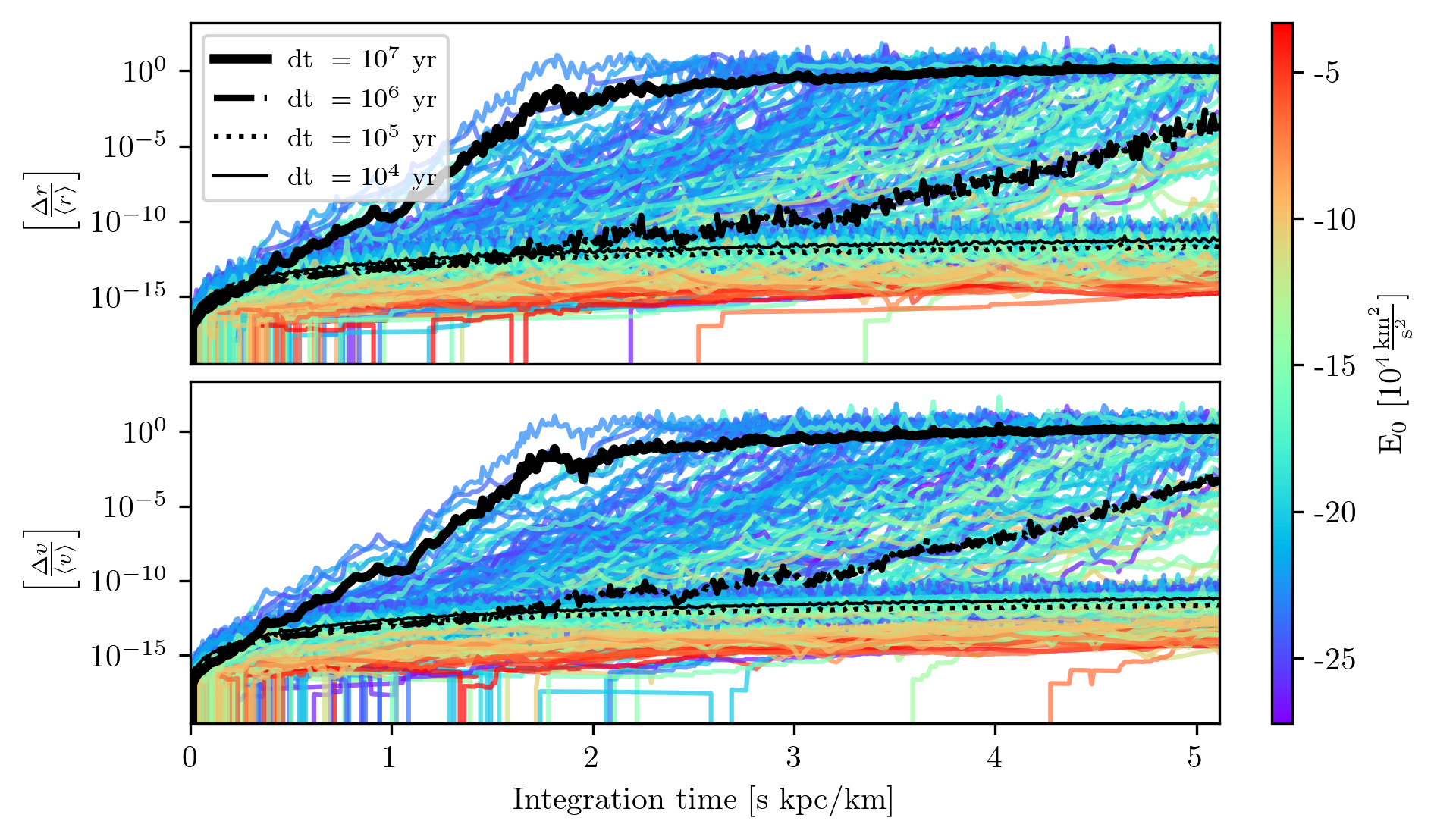
Fig. 2 illustrates the time reversibility of the integrator, i.e., its ability to retrace its own steps. For each timestep, I compute the difference between the forward integration and the backward retrace, normalizing to the mean of the two positions. The same computation is performed for the velocities. Specifically, I take the current kinematics of each cluster and integrate them forward in time for five billion years, storing positions and velocities at each step. Starting from the final state, I then integrate backward for the same duration, again recording positions and velocities at every step. At each corresponding time stamp \(t_i\), I calculate the vector differences in position and velocity, normalizing the positional error to the mean position of the forward and backward steps.
The timestep of \(10^7\) yr saturates only after 2 Gyr. The distances do not continue to grow because the orbital energy only differs by one part in ten, so at later timesteps, the cluster is still within the same region of phase-space, but the retrace is at a completely different location than the initial integration. The errors in the timestep of \(10^6\) yr become significant, though by the end of the integration period of 5 Gyr they are still only one part in ten thousand. The timesteps of \(10^5\) and \(10^4\) yr have excellent retraceability and on average, only differ by one part in \(10^{-14}\), and are thus only limited by round off error from the use of double precision floating point numbers.
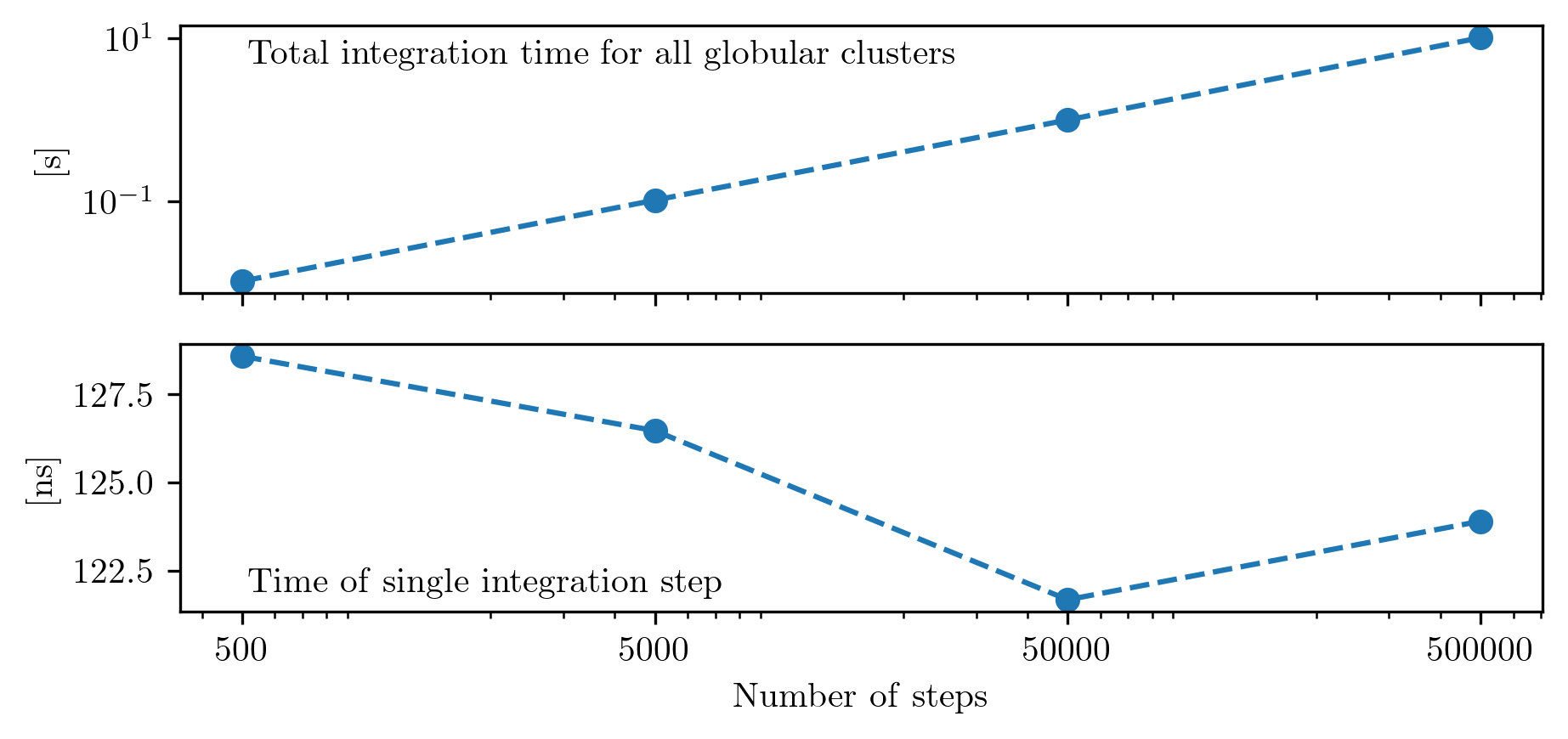
Computation time is quite important. Fig. 3 presents the total computation time of integrating the globular cluster system, and the time of a single integration step, which is computed by normalizing the total time by the number of objects and number of steps taken: \(T_{\mathrm{total}}/N_{\mathrm{GCs}}/N_{\mathrm{steps}}\). In general, the relationship is linear and the integration time per step per object is roughly constant. The downward trend presented in Fig. 3 is in part a coincidence, as some time realizations minimize this, and in part due to the overhead computation time with initializing and finalizing the calculation contributes less and less with increasing integration time. Nonetheless, for this processor (Apple M2 processor), for a single integration step the mean time is \(\sim\) 128 nanoseconds.
The Ruth-Forest algorithm discussed in the previous section was implemented and is reported in Fig. 4. Here, as expected, we see that the precision greatly increases when decreasing the timestep. However, since there are four force evaluations for a single timestep, this method is naturally slower per step than Leapfrog. How do the two methods compare over all?
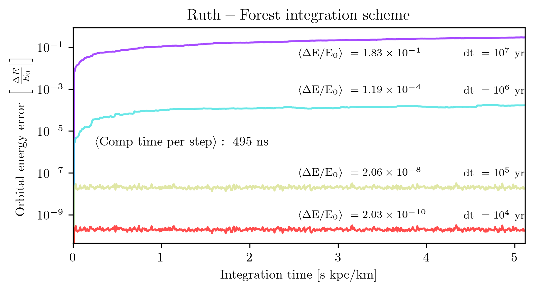
Fig. 5 compares the numerical error for again the total number of steps (which is inversely proportional to the timestep). It is clear that, for a given step size, the Ruth-forest outperforms the Leapfrog, but is it actually better? To answer this question, I fit the two curves with their own trend lines to find the number of steps required to have a relative error of \(10^{-8}\). With this requirement, The Leapfrog scheme requires 262,641 steps while the Ruth-Forest scheme requires 102,773 steps. However, given the difference in computation time per step, on average, the Forest-Ruth scheme takes \(\sim 1.5\)x more time for the same degree of numerical precision than the Leapfrog. For this reason, we use the Leapfrog algorithm. In this problem, numerical uncertainties are must less of a limiting factor compared to modeling uncertainties and observational uncertainties, so a better integrator for numerical precision is not worth the pay off of longer computation times.

A classic challenge in astronomy and the physical sciences arises when a problem involves two or more physical processes that operate on very different time scales. This is certainly the case when studying globular clusters. Figure 6 illustrates the orders-of-magnitude differences in time scales both across the globular cluster population and within individual clusters.
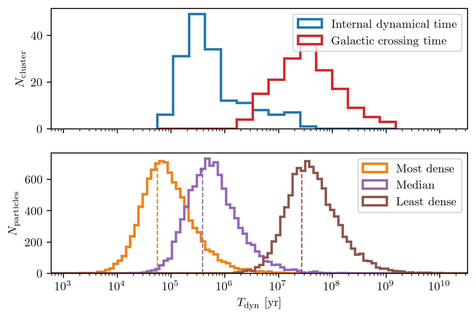
A useful metric for characterizing a system’s time scale is the crossing time, which is the time it would take a star to reach the center of the system given its current speed: \[t_\mathrm{cross} = \frac{r}{v}.\] While this quantity is not an integral of motion and varies as a star moves, it still provides a convenient and informative estimate of the dynamical time scale. It breaks down in extreme cases, such as a purely radial orbit near pericenter or apocenter where the instantaneous velocity approaches zero, but such cases are rare and do not undermine its utility. We compute the crossing time for each globular cluster in the galaxy (red distribution in the top panel of Fig. 6) as well as for each individual star particle within the clusters.
For the cluster as a whole, a robust characteristic dynamical time can be defined as: \[\tau = \sqrt{\frac{a^3}{GM}},\] where \(a\) is a characteristic size of the system. This is often taken to be the half-mass radius. In this work, I adopt the half-mass radius rather than the Plummer scale radius, though the two are related by \(r_{\mathrm{1/2}} \approx 1.3a\). This time scale was computed for each cluster and is shown as the blue distribution in the top panel of Fig. 6.
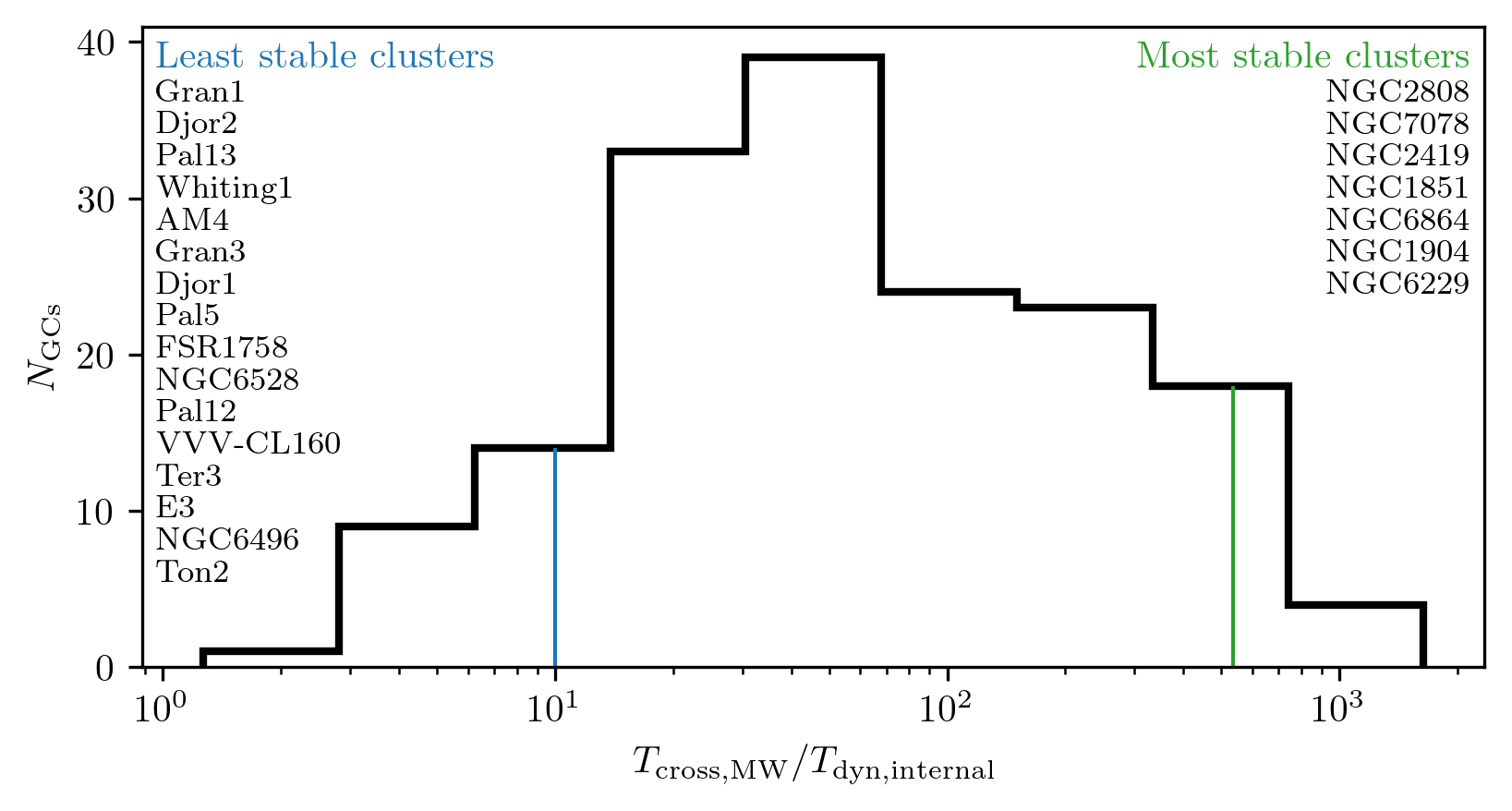
Note that the distribution of cluster dynamical times has a long tail toward longer values, overlapping with the galactic crossing times. A natural question arises: could any cluster have a longer internal dynamical time than its orbital crossing time? The answer should be no. If it takes longer for stars to orbit within the cluster than for the entire cluster to orbit the Galaxy, the cluster is effectively unbound or fully disrupted. I examined this question for the Galactic globular cluster population, and the results are shown in Fig. 7. As expected, all clusters have internal dynamical times shorter than their orbital crossing times.
Interestingly, the ratio of these two time scales serves as a useful diagnostic of cluster stability. Clusters in which stars complete hundreds or thousands of internal orbits per galactic orbit are significantly more stable than those where stars complete only a few.
To properly compute the orbits of the star particles, the timestep must be small enough to resolve the orbit accurately while the star is inside the cluster. How should we choose this timestep? There are two criteria. The first is that the timestep should be some fraction of the cluster’s dynamical time: \[\Delta t' = \alpha ' \tau.\] I use a prime to indicate that this is a trial timestep, since the second criterion must also be satisfied: the total number of timesteps should be an integer, \[N = \left\lceil \frac{T}{\alpha' \tau} \right\rceil,\] where \(T\) is the total integration time. We round \(N\) up to ensure a slightly smaller timestep, which becomes \(\Delta t = T/N\). This also redefines the effective timestep fraction as \(\alpha = \Delta t / \tau\).
In the experiments presented in this section, I choose several fractions of each cluster’s dynamical time and examine the resulting numerical errors. To efficiently explore a wide range of \(\alpha\), I begin with a few trial values of \(\alpha'\) and then round the number of steps down so that \(N\) is not only an integer, but also a power of two. This leads to the following condition: \[N = 2^{k-1}\] where \(k \in \mathbb{N}\) is an integer index. The expression for \(k\) becomes: \[k = \left\lceil \log_2\left(\frac{T}{\alpha ' \tau_\mathrm{dyn}}\right) + 1 \right\rceil. \label{eq:binary_time_step_criterion}\]
The goal is now to determine the appropriate value of \(\alpha\) to ensure energy conservation and time-reversibility. In the analysis presented in the previous sections, I selected timesteps without explicitly relating them to the crossing times of globular cluster orbits. Fig. 1 shows that a timestep of \(\Delta t = 10^4~\mathrm{yr}\) achieves a mean relative energy error of \(10^{-8}\). Meanwhile, Fig. 2 shows that a timestep of \(\Delta t = 10^5~\mathrm{yr}\) already achieves convergence in time-reversibility. Comparing these values to the typical crossing time shown in Fig. 6, we find that they correspond to \(\alpha\) values of approximately \(2 \times 10^{-4}\) and \(2 \times 10^{-3}\), respectively.
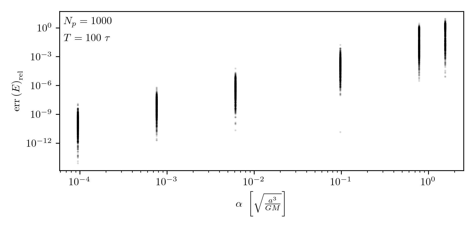
In Fig. 8, I investigate energy conservation in a static Plummer sphere using trial values of \(\alpha \in [10^{-4}, 10^{-3}, 10^{-2}, 10^{-1}, 1, 2]\). This experiment shows that values of \(\alpha < 10^{-2}\) yield excellent energy conservation. In this section, we do not consider the time-reversibility as the previous section has shown the integration’s robustness with regard to this metric. However, this is our main metric for the next section.
The preceding sections assessed the numerical stability of integrating globular cluster orbits within the Milky Way, focusing on time-reversibility and relative energy error across two integration schemes: Leapfrog and Forest-Ruth. I also considered the computational cost associated with different temporal resolutions. Separately, I evaluated the energy conservation for star particles evolving within a stationary Plummer sphere, quantifying the relative error as a function of timestep. In that context, the cluster’s potential was scaled to its scale radius, mass, and the gravitational constant. This non-dimensionalization allowed me to select timesteps as fractions of the internal dynamical time \(\tau\) of each cluster.
In this section, I combine them: I examine the quality of orbit integration for star particles evolving within a globular cluster, which in turn is orbiting in the Galactic potential.
I restrict the analysis here to the Leapfrog integrator for two main reasons. First, although the Forest-Ruth scheme achieves better energy conservation (see Fig. 5), this comes at a significantly higher computational cost, which outweighs its marginal gains for this application. Second, the equations of motion used to model stream generation require loading the position of the host cluster for each force computation. Because Forest-Ruth evaluates forces at non-uniform substeps, using it would require either: (1) storing and loading the cluster orbit at each substep, which would demand excessive disk space and complex code restructuring; or (2) interpolating the orbit at intermediate times, which introduces ambiguity regarding whether time-reversibility is preserved with linear or cubic interpolation. For these reasons, I opted not to explore Forest-Ruth further in the context of full stream generation.
To assess the performance of the stream-generation method, I designed a quality assurance experiment, illustrated in Fig. 9. I began by integrating the orbit of a globular cluster’s center of mass backward in time by 1 Gyr. At that point, I initialized a Plummer sphere with 512 star particles using the cluster’s half-mass radius and total mass. This system was translated to the center-of-mass phase-space coordinates and then integrated forward to the present day, forming a stream. I recorded the resulting positions and computation time. To test time-reversibility, I subsequently integrated the stream particles backward again for 1 Gyr.
A note on terminology: although the cluster orbit is initialized from present-day observations, in the context of stream generation, I refer to the past position (1 Gyr ago) as the “initial conditions”. The forward-integrated system represents the “stream”, and the backward-integrated version of the stream is referred to as the “retrace”.
Fig. 9 shows the results for four different timesteps. As expected, increasing the timestep degrades time-reversibility. For the largest timestep (\(\alpha \approx 1\), top left), the retrace fails to recover the original configuration. The retraced structure remains a stream and does not re-coalesce into a cluster. The results improve rapidly with decreasing timestep: at \(\alpha \approx 2 \times 10^{-1}\), most particles return close to their starting positions with only slight offsets. At \(\alpha \approx 2 \times 10^{-2}\), nearly all particles recover their initial conditions, and by \(\alpha \approx 6 \times 10^{-3}\), the retrace is nearly perfect.
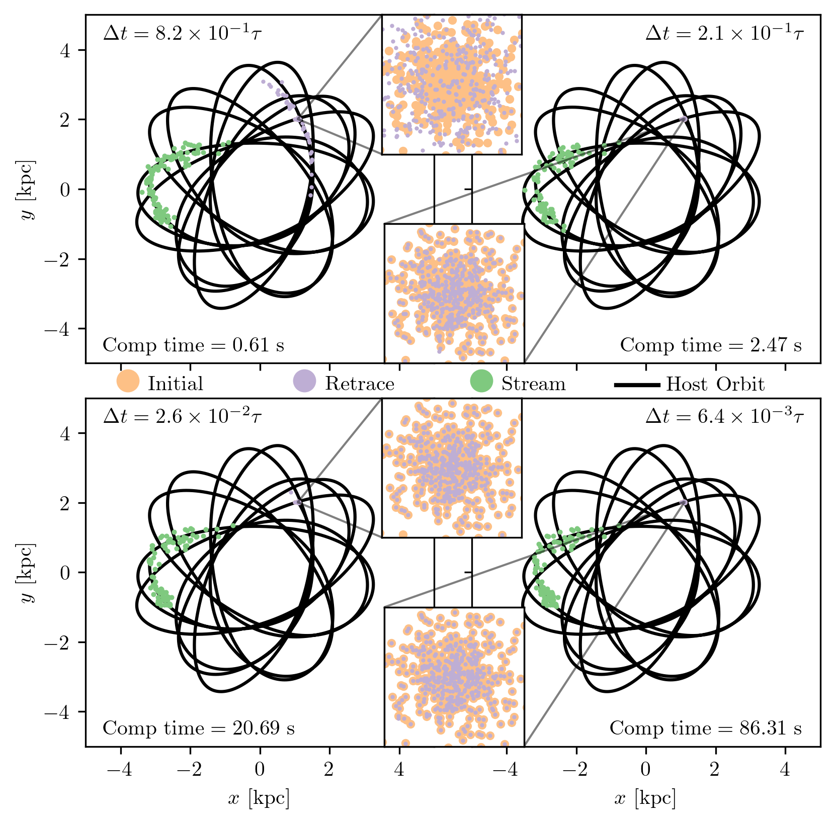
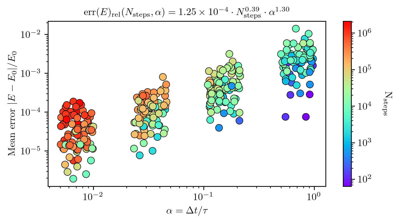
Fig. 10 presents the integrator’s energy conservation performance during the retrace phase of Fig. 9, across the same timesteps.
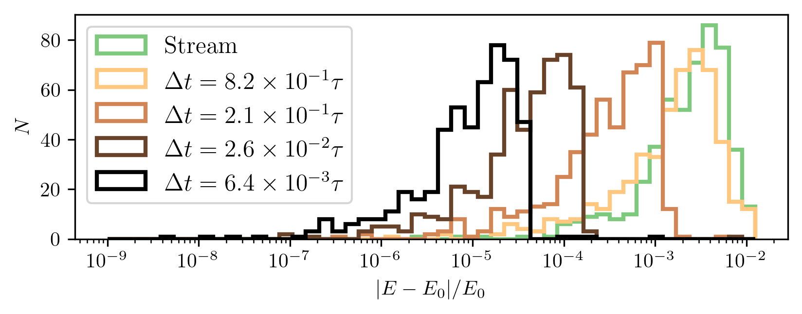
Although the retrace fails for the largest timestep in Fig. 9, Fig. 10 shows that the relative energy error remains modest—between \(10^{-4}\) and \(10^{-2}\). However, this metric requires careful interpretation. What appears as an “error” primarily reflects the intrinsic spread in orbital energies among star particles, relative to the center-of-mass energy.
We can estimate this ratio by comparing the internal potential energy scale of the cluster to its orbital energy in the Galaxy. The cluster’s characteristic potential is roughly \(\Phi \sim GM/a\), with \(M \sim 10^5~M_\odot\) and \(a \sim 0.005\) kpc, giving \(\Phi \sim 10^2~\mathrm{km}^2\,\mathrm{s}^{-2}\). Meanwhile, the typical orbital energy of a globular cluster is around \(10^5~\mathrm{km}^2\,\mathrm{s}^{-2}\).
This three-order-of-magnitude difference implies that the intrinsic energy spread from the Plummer sampling is about \(10^{-3}\) of the total orbital energy, which is consistent with the the apparent energy “error” in the stream of Fig. 10. Thus, this differences does not arise from numerical drift, but from the physical energy distribution encoded in the initial conditions.
Fig. 9 & Fig. 10 demonstrate the case of a single cluster. How is the energy conservation for the entire catalog? Fig. 11 presents the relative error in the conservation of energy for retracing the orbit of each individual star particle per globular cluster for each cluster in the catalog. Each data point reports the mean error in the conservation of energy. Each cluster was integrated for 5 Gyr. The upper limits for the timesteps were sampled logarithmically between \(10^{0}\) and \(10^{-2}\), the exact timesteps are based on the criterion from Eq. [eq:binary_time_step_criterion].
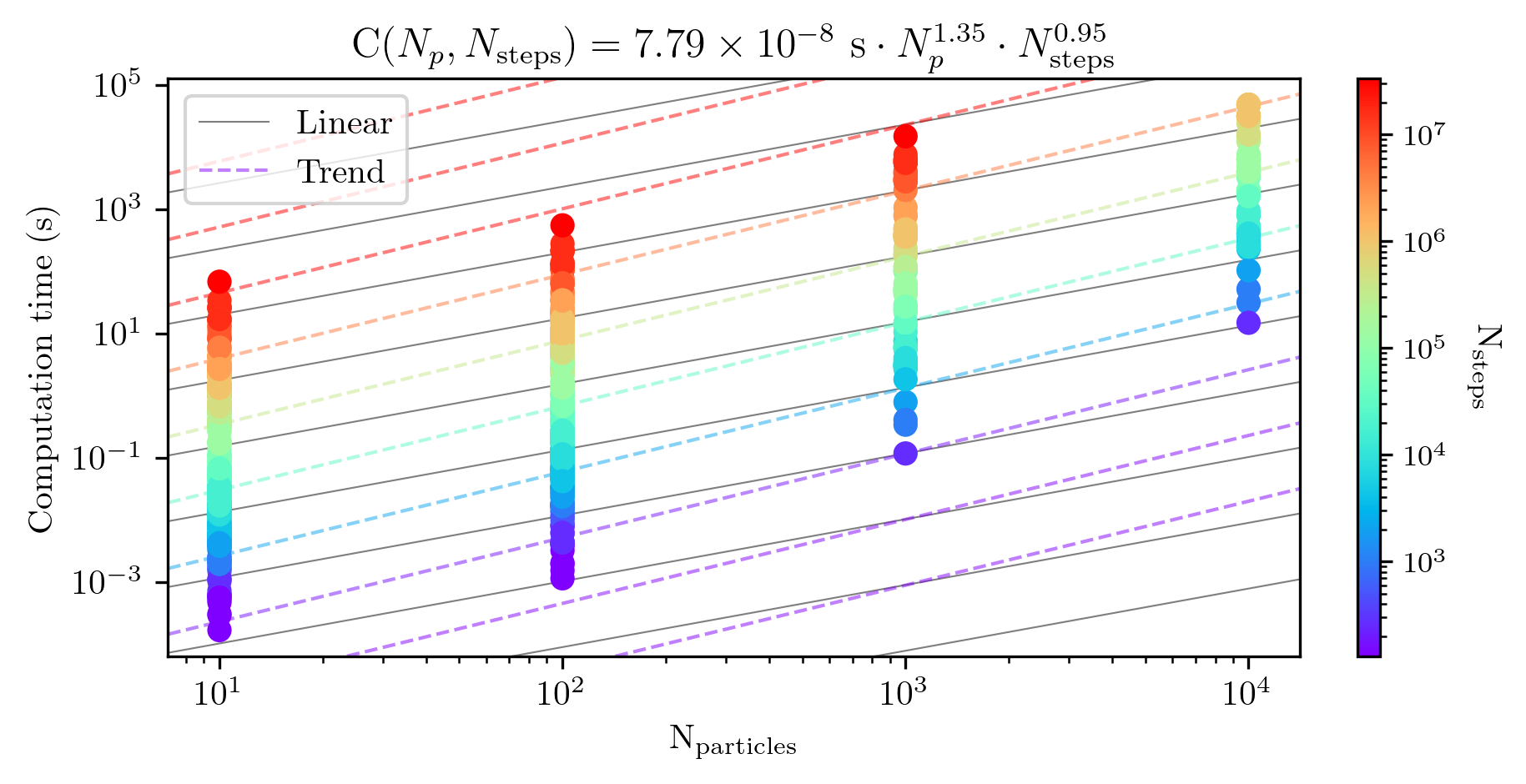
The quality of the solutions is fundamental for proper results. However, computation time and cost is also very important. The main motivation in using the restricted three body problem was to save computation time. With N body, the computation time should scale with \(N_p^2\), while for the restricted three body problem it should scale with \(N_p\). For both, it should scale linearly with the number of integration steps.
How does tstrippy perform? Fig. 12
presents the results from an experiment with all the globular clusters,
integrating them each for 1 Gyr. I choose the timestep to be at most
1/20 of each internal dynamical time, thus since each cluster has a
different dynamical time, it will require a different number of steps.
For each of these tests I use \(10^1,~10^2,~10^2,~10^3\) particles and
launched them on cluster at the Paris observatory. Then, I fit a scaling
law of \(C(N_p,N_s) = \langle C\rangle N_p^a
N_s^b\). If the code scales linearly, then each exponent, \(a,~b\), should be 1 and \(\langle C\rangle\) would be the mean
computation time.
Fig 12 shows that the code is less efficient than linear scaling with number of particles, since the best fit exponent is \(1.35\). However, it scales better than linear with the number of steps. Perhaps this can be explained by the fact that there is overhead time involved for initiating and ending each simulation. As the number of steps increases the fixed overhead proportionally takes up less of the total time. Since the power law has an exponent of \(0.95\), the overhead is marginal. However, it is fortunate that the exponent is not greater than 1, which would mean the code would slow down with execution time.
Putting Fig. 11 and Fig. 12 together, we may estimate for how long it completes to run these simulations. If we want all simulations to have error better relative error on the retraced conservation of energy than about 10\(^{-3}\), then we must pick timesteps that are smaller than about 1/20 of the dynamical time. With this criteria selected, we can compute the number of timesteps necessary for each globular cluster, which is a function of its internal dynamical time. By doing so, I find that the fastest cluster can be computed in \(\sim\) 30 minutes. The median computation time is \(\sim\)17 hours. The largest computation time was \(\sim\) 5 days. The total CPU time for the whole catalog is \(\sim\) 194 days.
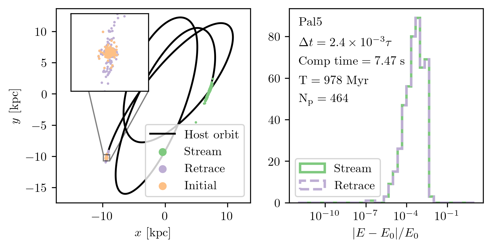
During the writing of this thesis, I discovered a bug in my code that affected the integration scheme. Specifically, the error concerned the way I handled the host orbit during the integration of the star particles. In earlier implementations, I would integrate the orbit of the host using the same timestep that I used later to integrate the orbits of the star particles. However, this approach violated the structure of the Leapfrog integration scheme.
In Hamiltonian integration, it is essential that the drift and kick steps alternate in a consistent manner. Since I implemented a drift-kick-drift (DKD) scheme, the kicks occur at the midpoint of each timestep, meaning that forces should be evaluated at intermediate positions. Previously, I erroneously computed the relative position vector as \[\Delta \vec{r}_i = \vec{r}_{p,i+1/2} - \vec{r}_\mathrm{GC,i},\] instead of the correct expression: \[\Delta \vec{r}_i = \vec{r}_{p,i+1/2} - \vec{r}_\mathrm{GC,i+1/2}.\]
This mistake appeared in both Ferrone et al. (2023) and Ferrone et al. (2025). Does this invalidate our results? To assess the impact, we can compare Figs. 13 and 10. In Fig. 13, the same retracing experiment was performed, but using the flawed integration: the host orbit was only provided at the same grid points as the stream. In the left panel, we see that the globular cluster does not perfectly re-coalesce when integrating backward in time, but the result is not catastrophic. Physically, we do not expect this process to be perfectly time-reversible; however, such irreversibility should ideally arise from physical modeling, not from numerical artifacts.
We also observe that the distribution of the relative error in energy conservation is nearly identical between the retraced and the original stream. In any case, once the stars move beyond the Jacobi radius, their dynamics are dominated by the galactic potential. Since this potential was integrated correctly and symplectically, the orbits of stars outside the cluster remain reliable and physically meaningful.
As a result of this discovery, I updated the tstrippy
code to warn users if the host orbit is not sampled at \(2N + 1\) points, where \(N\) is the number of integration steps.
While the flawed implementation breaks strict symplecticity for the
internal cluster dynamics, the Leapfrog integration for the globular
cluster orbits was still used correctly. This ensures that the cluster
center of mass returns to its present-day sky position and that stars
outside the cluster follow accurate galactic orbits. Ultimately, the
simplification of using a static Plummer sphere—whose mass and size
remain fixed—is a greater limitation than this particular numerical
error.
Lastly, I discovered this error while writing about the Forest-Ruth integration method. To implement this scheme correctly, I would need to know the position of the globular cluster’s center of mass at four intermediate points across two timesteps, with the spacing determined by the coefficients in Table 2. This would require either storing additional mini-time-step data or interpolating the globular cluster’s trajectory between saved snapshots. Both options would necessitate a substantial refactoring of the code or an impractical increase in memory usage per orbit. Given the results shown in Fig. 5, the gain in accuracy does not justify the computational cost.
This project is built on f2py, which allows integration
between Fortran and Python. The core motivation behind this choice is
performance: Fortran, as a compiled language, provides significantly
faster execution for numerically intensive tasks, while
Python—especially within Jupyter notebooks—offers a convenient
environment for development, experimentation, and visualization.
F2py stands for Fortran to Python (Peterson 2009),
and it is included as a module within NumPy (NumPy Developers
2025; Harris et al. 2020). The name of the project,
tstrippy, stands for Tidal
Stripping in Python.
F2py supports Fortran 77, 90, and 95 standards, so we
chose to write the code in Fortran 90 to make use of modules.
In Fortran, a module encapsulates data and subroutines in a manner
somewhat analogous to classes in object-oriented programming. However,
Fortran modules do not support inheritance, and only a single instance
of a module can exist at a time—unlike classes, which can be
instantiated multiple times.
Tstrippy package is structured around five core Fortran
modules, each responsible for a distinct aspect of the simulation:
integrator: This is the central module of the code.
It stores particle positions and velocities, computes forces, and
evolves the system forward in time. It also handles the writing of
output data at specified intervals and interfaces with all other modules
in the code.
potentials: This module defines the analytical
potentials used to compute gravitational forces. It currently supports
several models, including Plummer, Hernquist,
AllenSantillian, MiyamotoNagai, the bar model
LongMuraliBar from Long and Murali (1992), and the
composite model from pouliasis2017pii (Pouliasis, Di
Matteo, and Haywood 2017). This module can also be called in
Python, allowing users to call potential functions directly, e.g., for
computing energies during post-processing.
hostperturber: This module handles the host globular
cluster. It stores its orbit (i.e., timestamps, positions, and
velocities) and ensures its synchronization with the simulation’s
internal clock. It computes the gravitational influence of the host
cluster on each star particle. This is an internal module only.
perturbers: Similar in function to
hostperturber, this module supports additional perturbing
clusters. It allows for the inclusion of multiple perturbers and
computes their collective force on each particle. If object-oriented
programming were available in Fortran, both this module and
hostperturber would naturally inherit from a shared parent
class. This module only uses the positions, masses, and characteristic
radii of the other perturbers. The velocities are not imported.
galacticbar: This module stores parameters for the
bar, including the polynomial coefficients for its angular displacement
as a function of time: \[\theta(t) = \theta_0
+ \omega t + \dot{\omega} t^2 + \ddot{\omega} t^3 + \dots\] If a
user wants a bar with a constant rotation speed, then they may pass two
coefficients. If they want a bar that accelerates for decelerates, they
may mass more coefficients for the higher order terms. The module
performs transformations into the rotating bar frame, computes the
forces in that frame, and then transforms the forces back to the
Galactocentric reference frame.
This modular structure makes it straightforward to extend the code by adding new physics in the form of additional modules.
To make the package installable and easy to distribute, I initially
followed the guide by Bovy (2025b), which describes
how to create a Python package using setuptools—the
standard build system in the Python ecosystem. However, compatibility
between setuptools and f2py was broken
starting with NumPy \(>\) 1.22
(released June 22, 20222) and Python \(>\) 3.9.18 (released June 24, 20243). This meant that Fortran extensions
could only be compiled using deprecated versions of both. These older
versions of NumPy were also not compatible with Apple’s ARM-based M1 and
M2 processors, rendering the code unusable on modern Mac systems.
This limitation stemmed from the deprecation and eventual removal of
numpy.distutils, the tool that previously enabled seamless
integration of Fortran code in NumPy-based packages. As of NumPy 1.23
and later, numpy.distutils was deprecated, and with
NumPy 2.0, it was removed entirely. The NumPy developers recommended
migrating to meson (Meson Developers 2025) or
Cmake.
To address these issues, I migrated the build process to
meson, a language-agnostic build system capable of
compiling Fortran, C, and Python extensions across architectures. This
eliminated compatibility problems and made the build process
architecture-independent. The build system now automatically detects the
system architecture and compiles accordingly.
The code is fully open source and available on GitHub.4 To
support users, I created documentation hosted on
readthedocs.io5, which includes working
examples and basic usage guides. A minimal test suite, written using
pytest, is also included. While not exhaustive, the tests
ensure that core functionality remains intact as the code evolves. In
the next section, I present a minimal example of how the user may use
the code within a python script.
If the package is properly installed on the system, it can be imported at the top of any Python script:
Next, the user must load or define the initial conditions. The code provides:
The masses, sizes, and kinematics of the globular cluster catalog from Baumgardt and Hilker (2018);
The galactic potential parameters for model II of Pouliasis, Di Matteo, and Haywood (2017); and
A galactic reference frame.
The user must then select the system to integrate. For example, to
integrate the orbits of observed globular clusters, one must convert the
ICRS coordinates to a Galactocentric frame using astropy
and the provided MW reference frame. Alternatively, to simulate a star
cluster, one can generate a Plummer sphere:
Here, NP is the number of particles,
halfmassradius is the system’s half-mass radius,
massHost is the total mass of the Plummer sphere, and
G is the gravitational constant. All values must be in the
same unit system.
The integrator must then be initialized. All parameters are passed via lists that are unpacked at the function call. Here is an example of initializing the integrator for a stellar stream in a potential that includes a rotating bar:
setstaticgalaxy specifies the static potential model
and passes its parameters.
setinitialkinematics provides the initial positions
and velocities of the particles.
setintegrationparameters defines the initial time,
timestep, and number of steps.
inithostperturber specifies the globular cluster’s
trajectory and mass as a function of time.
initgalacticbar defines a rotating bar. It takes the
name of the bar model, potential parameters, and spin
parameters.
setbackwardorbit reverses the velocity vectors and
sets the internal clock to count down: \(t_i =
t_0 - i \cdot \Delta t\). For the usecase presented in this work,
setbackwardorbit is used for computing the globular cluster
orbits and not for the star-particles.
The user can choose between two output modes during integration:
Conceptually, these represent two output paradigms:
initwriteparticleorbits saves the full orbit of each
particle to an individual file.
initwritestream saves full snapshots of all
particles at selected timesteps.
Both functions take:
nskip: number of timesteps to skip between
outputs;
myoutname: the base file name;
myoutdir: the output directory.
The output files will be named like: ../dir/temp0.bin,
../dir/temp1.bin, ..., up to ../dir/tempN.bin,
where \(N = N_\mathrm{step} /
N_\mathrm{skip}\). Note that the files are written in Fortran
binary format. Although scipy.io.FortranFile can read them,
I use a custom parser based on numpy.frombuffer to avoid
the SciPy dependency. Once all parameters are set, the user can proceed
with integration using one of two methods:
leapfrogintime stores the full orbit of each particle in
memory. This is useful for a small number of particles or short
integrations—e.g., rapid parameter studies in a notebook. However, for
large simulations it can be prohibitively memory-intensive. For
instance, integrating all globular clusters at high time resolution
might require: \[7 \times N_p \times
N_\mathrm{step} \times 8~\mathrm{Byte} \approx 450~\mathrm{GB}\]
if \(N_\mathrm{step} \approx 10^7\).
This will likely exceed system RAM.
leapfrogtofinalpositions() performs the integration but
only returns the final phase-space coordinates. These arrays must be
copied before deallocating memory:
Deallocating is necessary to avoid memory leaks or crashes in Jupyter when rerunning code cells.
tstrippyThe earliest version of this code began as a simple Fortran script
that was interfaced to python via f2py and was built to
integrate test particles in specific gravitational potential models.
Since I was already familiar with Fortran and had working routines, I
chose to build on that foundation, gradually transforming the script
into a modular and more reusable package. Rather than switching to C++
or a Python-only solution, I continued using Fortran in combination with
f2py.
One of the primary motivations for writing my own code was
flexibility. When I attempted to implement a particle spray method in
Galpy, I found that performance degraded significantly when
using custom potentials not constructed from its internal C++ backend.
For example, I wanted to use the AllenSantillian halo
model, which is not natively supported. I followed the documentation and
implemented a class for it. However, custom potentials bypass
Galpy’s optimized C++ backend, resulting in slow
computations and rendering actions uncomputable (or at least with the
functions I tried). This pushed me to continue developing
tstrippy. I had a similar experience with
Amuse.
This choice, however, came with challenges. At one point, I tried implementing potentials derived from exponential density profiles, which do not admit closed-form solutions for the potential. I attempted to work in elliptical coordinates, motivated by the idea that the potential would depend only on the “distance” from the center along the equipotential surfaces. While I successfully implemented simple potential models in elliptical coordinates, I naively overlooked that this changes the equations of motion entirely due to the underlying geometry. I found that my orbits always diverged (except in special cases). It was only later that I realized I would need to account for the metric tensor and Christoffel symbols to properly integrate orbits in elliptical coordinates. At that point, I chose not to pursue this further, prioritizing scientific analysis and launching other simulations instead. This experience helped me appreciate why many codes and other published works prefer basis function expansions for such problems. In hindsight, this episode was a perfect example of how even unsuccessful attempts can lead to valuable insights. Below, I summarize some of the key advantages and limitations I encountered while developing a code from scratch to answer a scientific question.
Developing and maintaining this codebase brought several clear benefits:
Understanding. Writing the code forced me to deeply understand the modeling techniques involved. Otherwise, the results would have been incorrect.
Flexibility. I could implement exactly the models I needed and extend them as required.
Transparency. Results produced by my code can be verified and reproduced by others.
Reusability. Ongoing development helped me uncover and fix subtle bugs (e.g., related to non-symplectic integrators) that do not trigger obvious errors and only appear in edge cases or after close inspection. Long-term engagement with the code is key to catching these issues.
Collaboration. A fellow researcher at the Paris Observatory is now using the code. I also used it to supervise a master’s student during their semester research project, something that would not have been possible without building a user-friendly tool.
Growth. This project pushed me to adopt best practices:
version control, documentation, modularity. Developing my own code has
also made it easier to understand external libraries. For example, when
I implemented the King model, I studied Galpy’s internals
to cross-check my own method. I was delighted by how much easier it was
for me to use, despite the fact that I had not touched it within a
year.
However, there were also drawbacks:
Time cost. Developing the code took time away from direct scientific analysis. It’s possible I could have performed more simulations or performed more analyses had I not develop my code to such an extent.
Feature limitations. My code still lacks capabilities present in other packages: such as basis function expansions, action-angle variable computation, or parallelization strategies using MPI or OpenMP.
Changing relevance. Scientific priorities and available tools evolve rapidly. A general-purpose tool may become obsolete more quickly than a single-use script written for a specific question.
Compatibility and maintenance burden. Making the code
accessible to other users also introduces challenges related to
cross-platform compatibility and dependency management. Software
environments evolve, compilers are updated, dependencies can deprecate,
and build tools change. Even with the help of modern tools like
meson or f2py, ensuring continued
compatibility requires regular testing and adaptation. As the codebase
grows, the maintenance load increases, and sustaining it as a single
developer becomes increasingly difficult, especially if the tool is made
too general.
Nonetheless, the code was designed to address concrete scientific questions about Milky Way stellar streams and globular clusters. In the next two chapters, I present how this tool contributed to advancing our understanding of the Galaxy.